Mobile Air Quality Sensor
Abstract
Air quality is a measure of its suitability for breathing. Good air has a low concentration of particles and chemical pollutants, excess of which can cause long-term and short-term adverse health effects. Measurements of air quality are crucial for making informed decisions. However, current practices of monitoring air quality could improve their spatial and temporal resolution. These limitations, in turn, limit precision in decision-making. Low-resolution measurements also limit analytical models used for planning and design. Although higher resolution measurement is possible, it is constrained by its cost, deployment time and engineering impracticality. This report explores potential solutions for understanding air quality at a higher spatial resolution without these limitations.
Background
Pollution occurs when harmful concentrations of particles, liquids and gases are introduced into the environment (Manisalidis, Ioannis, et al.) Unfortunately, as the world develops and access to clean fuels or technologies remains limited, the air will become more polluted. Consequently, avoiding exposure to areas with bad air quality is challenging, whether from ambient air or household air pollution. Widespread exposure has short and long-term health effects. For example, the World Health Organization estimates that “nine out of ten people breathe polluted air.” EHINZ reports 3,317 premature deaths, representing 11% of all deaths in New Zealand in 2016.
Causes and Effects of Bad Air Quality
Air Quality Taxonomy: Pollutants and Factors
Particulate Matter
Particulate matter (PM) are solid and liquid particles in the air, ranging in size but small enough to be inhaled by humans. The most common sources of particulate matter are domestic fires and motor vehicles (EHINZ). Particulate matter smaller than 10 micrometres can penetrate the lungs. Finer particles less than 2.5 micrometres can be absorbed into the bloodstream (Ministry for the Environment).
Volatile Organic Compound (VOC)
Volatile organic compounds (VOCs) are chemicals that easily vaporise in air and dissolve in water. Using automatic insect spray dispensers, cleaning products, and building materials like paints, solvents, and adhesives has increased the concentration of volatile organic compounds in indoor areas (Manisalidis et al.). At the same time, heavy industry emissions also contribute to ambient air VOCs.
Carbon Oxides
Carbon dioxide and monoxides are products when a reactant undergoes combustion, like in gas stoves, engines or industrial processes. Although harmless, higher carbon dioxide concentrations reduce the oxygen available for inhalation. Meanwhile, carbon monoxide binds to haemoglobin, preventing oxygen exchange and transport. The carbon monoxide bond is approximately 250 times stronger than the oxygen bond with haemoglobin (Carbon monoxide poisoning). Therefore, while carbon dioxide is relatively harmless at low concentrations, carbon monoxide can be hazardous even at low levels of exposure.
Temperature and Humidity
The temperature in space will affect the variance in air quality (UCAR) due to the properties of gases and thermodynamics. Warmer air rises near the ground, and colder air sinks. This process moves pollutants from the floor to higher altitudes. Therefore, the temperature gradient of a space is directly proportional to the variance in air quality, as it affects the rate at which pollutants rise and fall. Furthermore, greater humidity reduces air circulation, which means more pollutants are trapped in the air (How does humidity affect air quality? all you need to know).
Causes
There are several causes and sources of bad air quality. Ambient sources of air pollution include vehicle emissions, industrial activities, dust, and wildfires. These sources emit particulate matter, nitrogen oxides, and volatile organic compounds. For instance, wildfires can release significant amounts of particulate matter (Wiedinmyer C. et al.), and industrial activities release volatile organic compounds and particulate matter. With the increase in global temperatures, wildfires are becoming more common. There have already been twenty-three wildfires since 2023 (Wildfires in 2023).
However, the problem is not limited to ambient sources; household sources can also cause bad air. Cooking, heating, smoking, building materials and cleaning products are common sources of indoor air pollution. Gas stoves and heating appliances release carbon, nitrogen, and particulate matter oxides. In contrast, tobacco smoke emits volatile organic compounds and particulate matter. Even e-cigarettes, often touted as a safer alternative to traditional cigarettes, produce aerosols containing nicotine and particulate matter and “low levels of toxins that are known to cause cancer” (Electronic smoking devices and secondhand aerosol - American nonsmokers’ rights foundation). Building materials and cleaning products may also emit volatile organic compounds.
Effects
Inhaling bad-quality air can have short and long-term adverse health effects.
Particulate matter, which can easily penetrate our respiratory defences, can irritate the eyes, throat, and lungs in the short term while worsening existing respiratory conditions like asthma (Why Air Quality Matters). Long-term exposure to particulate matter increases the risk of cardiovascular diseases, lung cancer and infant mortality (How air pollution is destroying our health).
The effects of volatile organic compounds are less well known, given the variety of these compounds. However, common short-term effects may include irritation of the eyes, nose and throat. In contrast, prolonged exposure may involve toxic reactions (Terry Gibb).
Finally, the short-term effects of oxides of carbon are similar. People temporarily exposed to high concentrations of carbon oxides may experience headaches and dizziness. Brief exposure to carbon monoxide may also cause nausea, leading to vomiting and, finally, a loss of consciousness. If people are exposed to carbon monoxide for extended periods, “hypoxia, ischemia, and cardiovascular disease are observed” (Manisalidis et al.).
Exposure to bad air can also reduce attention span, memory recall and concentration.
Consequently, it is estimated that one-third of deaths from stroke, lung cancer and cardiovascular disease are due to exposure to air pollution (How air pollution is destroying our health). In New Zealand, poor air quality is responsible for around 13,000 hospitalisations and cases of childhood asthma (EHINZ).
Air pollutants can settle onto land and water, which plants and animals will absorb. These pollutants will impede plant growth and affect animals the same way they affect humans. Furthermore, these contaminants will eventually end up in humans as they inevitably work up the food chain or through drinking water. High concentrations of bad air may also reduce visibility by scattering or absorbing light, potentially increasing the chances of accidents (Ministry for the Environment).
Stakeholders and Concerns
Government
The government plays an essential role in decision-making. They are responsible for allocating resources and programs to promote healthy living and prevent unnecessary strain on the healthcare system. It is estimated that “the global cost of health damages associated with exposure to air pollution is $8.1 trillion” (World Bank.) The local and national government’s policies directly affect those under their jurisdiction. Therefore, this stakeholder must obtain high-resolution data to make informed decisions on effectively allocating resources.
Education Institutions
Schools are also critical stakeholders since they significantly impact children’s health and well-being. Children are among the most vulnerable stakeholders to the impacts of long-term exposure to polluting air. The United Nations Framework Convention on Climate Change estimates that “polluted air affects more than 90% of children”. With high-resolution air-quality data, schools may make precise decisions that improve their students’ health and alter their activities accordingly.
Companies
In most countries, there are laws to ensure employers protect their employees’ and clients’ health and safety, though to varying extents. Companies can assess the impact of air pollution on their operations and take steps to mitigate it with high-resolution air quality data. This can improve their working environment and customer satisfaction, benefitting the business’s operations. Even from an altruistic perspective, high-resolution data may allow some corporations to differentiate their products and services from competitors and make the claim of having a service with a more significant positive environmental impact. This may attract environmentally conscious consumers and employees, gaining a larger market share.
Individuals
People should be able to make informed judgements since breathing polluted air harms their health. Children and the elderly are the most vulnerable (World Health Organization). Individuals can lower their risk of health problems by making informed decisions regarding their activities and pollution exposure.
Problems with the Current Solution
It is significant to clarify that this paper does not concern any solutions for reducing poor air quality or extensive analysis of potential actions stakeholders can take if they acquire such data. It offers some initial concepts to illustrate the feasibility of utilising high-resolution measurements. Instead, this paper proposes a solution regarding how such data is gathered. The decision to use the data collected is up to the stakeholder.
Assumptions
The cost-benefit analysis of the solutions considers four factors: monetary cost, technical feasibility, practicality and potential externalities. The monetary cost will be the cost of purchasing sensor unit(s), which is approximately $108.03 per unit (refer to the table below), along with the linkage cost. The technical feasibility will consider the cost of data storage and alternative solutions, such as using WIFI to transmit data instead of linkage. Practicality is evaluated by considering deployment time, whether or not sensor units will interfere with useable space and if it is possible to repurpose the sensors for outdoor space usage.
The following table provides a comprehensive breakdown of the costs associated with each component to estimate each potential solution’s monetary cost.
| Item | Price |
|---|---|
| Linkage | $0.60 / m |
| Arduino UNO (microcontroller) | $48.20 / unit |
| DHT22 (temperature and humidity sensor) | $2.55 / unit |
| MHZ19 (CO2 sensor) | $28.73 / unit |
| PMS5003 (particulate matter sensor) | $22.86 / unit |
| MQ135 (VOC Sensor) | $1.77 / unit |
| DS3231 (real-time clock) | $3.32 / unit |
This table lists some assumptions made about the sensor and indoor room volume.
| Parameter | Value |
|---|---|
| Average Room Volume | 8m × 10m × 3m = 240m³ |
| Effective Sensor Unit Coverage | 0.3m × 0.3m × 0.3m = 0.027m³ |
The four factors considered will not exhaustively represent every variable, and some crucial aspects may have been omitted or simplified. Nonetheless, these factors will provide a general idea in determining the feasibility of potential solutions and identifying potential bottlenecks that could hinder its success.
Current Practice
Description
The current practice for measuring air quality is installing a single sensor per room or a single sensor to cover every unit space for outdoor locations. While this approach has several advantages, it also has a significant limitation.
Advantages
One key advantage of this approach is that it is the most economical solution. Each sensor unit will cost approximately $108.03, with negligible wiring costs. Furthermore, this results in negligible technical issues. In an average home, there is enough WIFI bandwidth and channels for the sensors to send data to the cloud. If the data is stored locally, the low sensor count means data storage of sensor data will be negligible. Consequently, the current practice can afford a high temporal resolution due to the low storage cost. These sensors are relatively small and do not interfere with usable space, making them aesthetically pleasing.
Disadvantages
However, as mentioned in the assumptions, an air quality sensor’s adequate sensor unit coverage is 0.026m³. This means the air quality of an entire space will be approximated and does not accurately represent the quality across the space. The spatial resolution of the sensor is limited.
Why is High Spatial Resolution Important?
Spatial resolution matters as air quality can vary significantly across space due to various factors. The location of pollution sources and how the pollutants move across the space means different areas will be more concentrated than others. This means that depending on the location of the mounted sensor, there is a chance of detecting false positives, even though the air quality elsewhere is fine, or false negatives, where the air quality detected is fine but elsewhere is not. This problem only scales up with space volume. The lack of spatial resolution hampers the ability to pinpoint specific areas of bad air. Identifying local pollution sources and areas will be challenging.
Different stakeholders require high-resolution data for different reasons.
Governments are responsible for allocating resources and programs to promote healthy living and prevent unnecessary strain on the healthcare system. The local and national government’s policies directly affect those under their jurisdiction. High-resolution measurements of air quality data mean that government and local councils can identify the sources and patterns of air pollution in different areas and, at times, precisely map and identify pollution “hotspots”. This allows them to implement measures to reduce emissions, such as building green spaces in areas with high concentrations of pollutants. These measurements also allow the government to evaluate their green policies’ effectiveness precisely. Furthermore, the data gathered can be extrapolated to inform the public about current and forecasted air-quality levels and advise them to avoid certain areas, stay indoors or wear masks. This idea can be extended to targeted messaging of vulnerable groups.
Schools are responsible for the children’s health. Schools can utilise high-resolution measurements to improve students’ health. The data can inform schools regarding the suitability of outdoor activities or the need to adjust ventilation in classrooms, gymnasiums or changing rooms. At a minimum, it can inform the schools when and when not to open windows to improve indoor air quality. Schools can use this data to identify and adapt the ideal learning environment.
Companies are responsible for their employees’ and clients’ health. High-resolution data benefits businesses as it allows them to identify and resolve sources of pollution, resulting in a healthier and potentially more productive workforce by reducing health issues stemming from poor air quality. Services can gather high-resolution air quality data, which can help promote greater accountability regarding environmental regulations. Furthermore, high-resolution data can foster innovation, allowing businesses to create goods and services that aim to address air quality concerns.
Finally, individuals should be able to make informed judgements since breathing polluted air harms their health. High-resolution measurements mean they can plan their activities according to their location’s current and forecasted air quality levels. It can inform individuals whether or not to wear masks, use air purifiers, stay indoors when there is terrible air or even where to avoid in a building or outdoors.
Are There Air Quality Variances in Space?
A case has to be made on whether or not air quality varies between spaces and times. A portable sensor unit can be constructed and manually conduct systematic air quality measurements across different spaces. Analysing the data will enable us to determine the extent of variance in air quality across space, observe potential patterns and determine whether or not it is necessary to pursue further research and solutions.
The table below is a brief overview of the components. The portable sensor unit’s design, testing and integration will be discussed in Appendix A.
| Component | Function |
|---|---|
| Microcontroller | Reads sensor data and saves data to SD card |
| Temperature and Humidity Sensor | Records temperature and humidity |
| CO2 Sensor | Records CO2 concentrations |
| VOC Sensor | Records VOC concentrations |
| Real-Time Clock | Records time stamps for data logging |
| SD Card Reader | Interfaces SD card with microcontroller |
Various sensors are continuously collecting diverse data points. A pollution concentration index derived from a weighted combination of sensor readings will serve as the benchmark to assess relative air quality in different environments. The formula gives the pollution concentration index:
\(\text{PCI} = \begin{bmatrix} 0.05 & 0.2 & 0.5 & 0.1 & 0.7 & 0.4 & 0.3 \end{bmatrix} \cdot \begin{bmatrix} \text{Temperature} \\ \text{Humidity} \\ \text{VOC} \\ \text{CO2} \\ \text{PM1.0} \\ \text{PM2.5} \\ \text{PM10} \end{bmatrix}\)
By recording timestamped GPS coordinates from the phone, it is possible to match the sensor data with location information. Air quality data has been gathered from the following locations: home, school and hardware stores.
Data gathering and processing will be discussed in Appendix B.
Home
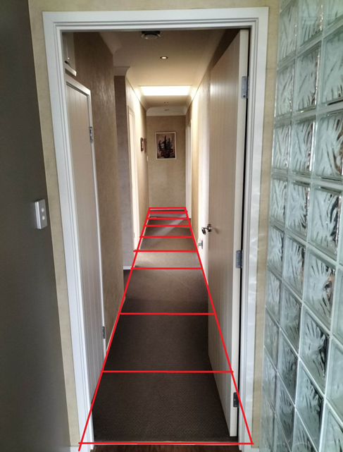 The air quality measurements at home resulted in the following pollution concentration index. The sensor took periodic readings at each section, marked by the red grids in the photo. For graph understanding purposes, section one is the red box the furthest away from the camera, and section eight is the red box closest to the camera.
One critical detail to note is that the air quality readings were taken when cleaning was happening around the house. This home measurement aims to see if there are variances in air quality in adjacent spaces. If the hypothesis is confirmed, we should see significant changes in the pollution concentration index due to changes in VOC for easy analysis. We should expect the pollution concentration index to remain steady if there are no air quality variances.
The table below is the average data for each section.
| Temperature (°C) | Humidity (%) | VOC PPM | CO2 PPM | PM1.0 (ug/m³) | PM2.5 (ug/m³) | PM10 (ug/m³) | PCI |
|---|---|---|---|---|---|---|---|
| 22.28 | 61.31 | 266.88 | 1399.85 | 0.05 | 0.05 | 2.90 | 287.726 |
| 22.44 | 60.95 | 248.52 | 1026.65 | 0.00 | 0.45 | 2.95 | 241.302 |
| 22.61 | 60.64 | 295.82 | 1209.35 | 2.00 | 6.15 | 6.15 | 287.8085 |
| 22.82 | 60.45 | 417.71 | 881.60 | 0.35 | 3.90 | 3.90 | 313.221 |
| 23.04 | 59.85 | 459.84 | 761.55 | 1.00 | 1.35 | 1.35 | 320.842 |
| 23.21 | 60.01 | 927.60 | 729.10 | 0.55 | 1.85 | 3.35 | 552.0025 |
| 23.40 | 59.75 | 1256.28 | 825.60 | 4.10 | 8.85 | 9.75 | 733.155 |
| 23.61 | 58.71 | 1354.25 | 774.65 | 1.60 | 4.25 | 6.20 | 772.1925 |
| 23.79 | 57.72 | 838.60 | 677.00 | 1.15 | 2.65 | 3.75 | 502.7235 |
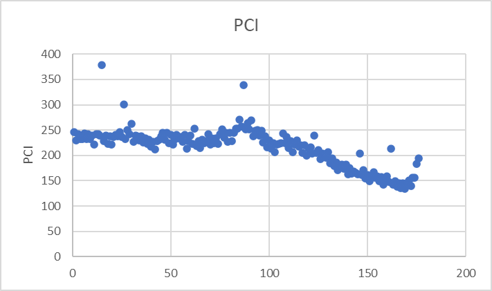
The graph below shows the variances in the pollution concentration index.
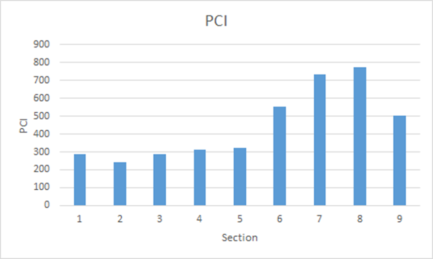
The graph notes that the pollution concentration index from sections one to five remains constant. However, from sections six to nine, there is a sudden change in the pollution concentration index. This shows that there are variances in air quality within space. This corresponds to what was happening on that day as well.
Section six is next to the bathroom. The bathroom was cleaned a few minutes ago with chemicals that contain volatile organic compounds. The table shows that the volatile organic compound concentration doubled, from 459.84 ppm to 927.60 ppm.
Section seven is next to the laundry room, where all the volatile organic compounds are stored and used. The sensor has correctly measured a further increased concentration of volatile organic compounds.
Sections eight and nine started approaching the wooden floor not shown in the picture. The chemicals were also used to clean the wooden floor, and the air quality measurements reflected this.
The lack of temperature, humidity and carbon dioxide variances is trivial and requires no analysis. However, there is no clear explanation for why particulate matter concentrations vary. One possible explanation may be that this area has been vacuumed before measurement, which may have disturbed the dust particles.
This experiment has proven that there can be variances in air quality within a small space. However, due to the unique experimental conditions (during cleaning), variances in air quality are almost guaranteed. In most cases, there may not be a drastic difference in air quality in small spaces; therefore, further testing and analysis must be conducted.
Hardware Store and Auto Parts Store
The point of this investigation is to see whether or not there are variances in air quality for large indoor spaces. A hardware store was chosen as businesses were one of the essential stakeholders discussed before. It is a well-known fact, and from personal experience, that hardware stores have less-than-ideal air quality conditions. However, no work has been done to quantify it.
The air quality measured will be at a large hardware store franchise and the auto parts store next door.
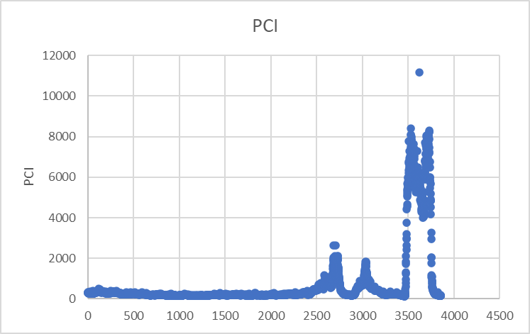
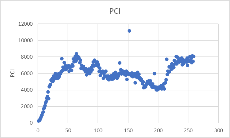
The auto parts store primarily sells various chemicals (volatile organic compounds). From the graph above, it is reasonably apparent which sections represent auto parts stores. The pollution concentration index peaked near 11600. The space outside had a pollution concentration index of around 200. This meant the air quality within Supercheap Auto was approximately sixty times worse than outdoors. Due to the abnormal, though expected, values of auto parts store, most data points are no longer visible. Therefore, A more detailed analysis should be conducted at a more micro-scale. The graph will be split into four sections: the pollution concentration index inside the hardware store, the walk to the auto parts store, the auto parts store, and the outside of the auto parts store.
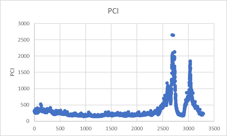
Inside the hardware store, there are two noticeable peaks. The two peaks identified from the data processing pipeline were when the sensor was at the woodworking section. The high particulate matter concentration from all the wood dust led to a high pollution concentration index.
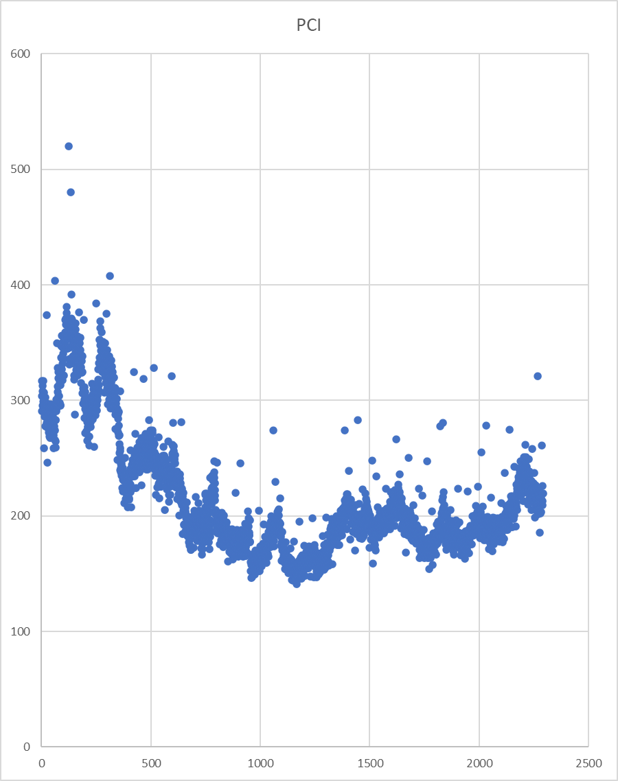
However, these two abnormal peaks meant other data points became invisible. Removing the two peaks and analysing points 0 to 2400 yields hidden details. As seen in the graph below, there seems to be a periodic increase in the pollution concentration index. This pattern proves there are variances in air quality in small spaces.
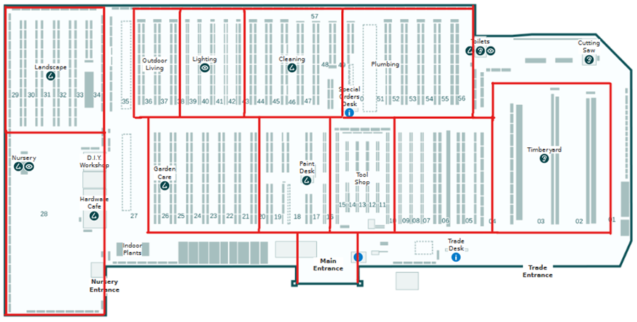
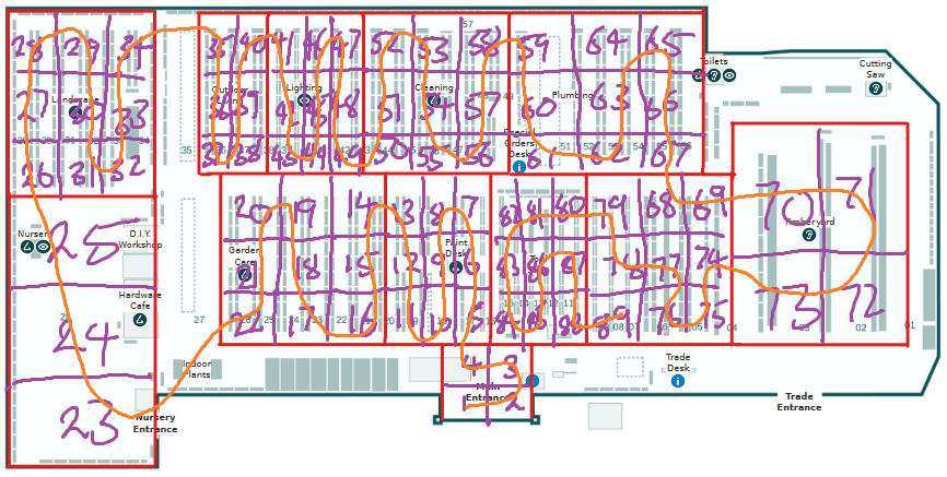
On further analysis, the periodic difference in air quality can be justified by the layout of the hardware store. As mentioned in Appendix B, the sensor moved across the aisles, as seen in the store map.
Traversing each aisle within the hardware store reveals a distinct pattern in the concentration of airborne pollutants, characterised by an initial ascent, a peak concentration at the midpoint, and a subsequent decline. Conversely, due to enhanced air circulation, the sensor’s exposure to pollutants is notably limited when progressing across the aisles within communal areas. This discrepancy can be attributed to the enclosed nature of traversing aisles, wherein the sensor becomes enshrouded by more pollutants. As one enters the aisle, the envelopment of pollutants around the sensor remains relatively constant due to the constrained measurement area. However, the air inflow from the shared space between aisles decreases when one walks further into the aisle—consequently, the pollution concentration increases. With this logic, we should expect the centre of the aisle (the location that experiences the least airflow, as it is furthest away from the shared space) to have higher concentrations of pollutants. Upon walking towards the aisle’s exit, analogous principles apply, akin to the conditions observed upon initial entry. The pollution concentration index graph supports this hypothesis. Matching the data points of one of the periodic readings with the location information confirmed this theory. The data essentially confirms that there are variances in air quality, even in small spaces.
The air outside the hardware store while walking towards the auto parts store remained relatively constant.
Not much data analysis is required for the auto parts store. This is because the pollution concentration index is so large that any variances in the air quality inside the store have little to no effect.
As the sensor left the auto parts store, the PCI immediately decreased, eventually converging to 250. This meant the air outside the auto parts store was approximately the same as outside the hardware store. This may initially seem counterintuitive given the high concentration of pollutants in the auto parts store; however, it is expected behaviour. Inside the auto parts store, there was barely any ventilation. This meant it was hard for the volatile organic compounds to diffuse into the surroundings unless the door was opened.
School
The point of this investigation is twofold: to see whether or not there are variances in air quality in outdoor spaces and to see whether or not there are variances in air quality indoors under normal conditions. The home experiment only showed variances during cleaning. This investigation will measure air quality during a typical day. Schools are one of the essential stakeholders.
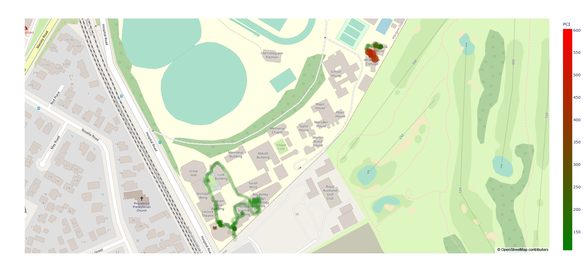
From the image above, it is clear that there are distinct sections of drastically varying air qualities in a large area. A more detailed analysis should be conducted at a more micro-scale. At the macroscale, there will always be variances in air quality.
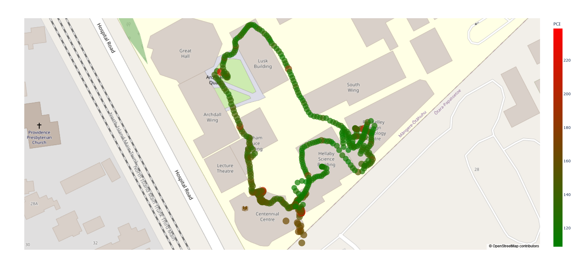
The trail on the map shown is all the data points the air quality sensor measured when walking around the central area of the school. To interpret the data, the redder the point is, the greater the pollution concentration index, the worse the air quality. From the picture above, it can be noted that there are distinct sections with variances in air quality.
Starting from the top left corner, around the Great Hall area, there is a distinct red point surrounded by off-green data points. This coincides with what is happening, which is the construction of a new building in that area. Following the data points around the Lusk building, the air quality gradually improves as it becomes further away from the construction. However, there is a single point of bad air, which could not be explained.
The next section of bad air quality is around the technology building. Again, this coincides with reality as there is much woodworking in the technology building, thus higher particulate matter concentrations. Although this graph does not show this, the sensor measured values of the art department, which is on the third floor of the technology department building. The paints may have contributed to less-than-ideal air quality in this section.
Finally, the air quality was consistently worse around the Centennial Centre than elsewhere. However, the source of pollution could not be pinpointed. A hypothesis of why air quality is terrible around here may be because it is relatively close to Hospital Road. This means car emissions may drift towards the school. This hypothesis is partially supported by the fact that subsequent data points close to Hospital Road are distinctly worse than those far away. This is particularly concerning for pre-schools near busy roads if this is the case. As discussed previously, younger children are at risk.
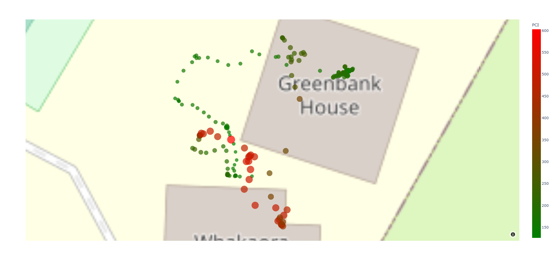
Analysing the Greenbank area, we notice less-than-ideal air quality around certain areas inside the house. From the image, the left side of the house, where the bad air is, is the bathroom and the lockers. Other places inside the house are fine.
The place of concern is the area outside of the house. However, nothing was noteworthy to justify the immediate increase in air quality. Since the air quality sensor has consistently shown expected data, the most likely explanation is that there may be an error in the GPS. GPS has an error of around 5 meters. However, if this were a GPS error, the air quality measurements would correspond to spaces inside the house, which is equally concerning.
Vertical Dimension
The point of this investigation is to determine whether or not air quality varies with height. If it did not, proposed solutions do not need to consider the third dimension, increasing simplicity and reducing cost. However, due to time constraints, the experiment has not been carried out with the sensor. According to the literature, air quality does vary with height due to turbulence and other factors (Aristodemou et al.; Lee et al.) Therefore, it is worth investigating the vertical dimension.
Conclusion
Through this investigation, one can confidently argue that indoor and outdoor air quality variances exist. Indoor air quality does not vary as much during everyday use. It will only vary if other factors exist, such as ongoing cleaning. However, if we look at different places indoors, there are still noticeable changes in air quality. The air quality in the Lusk building is very different from the air quality in the technology building, which also differs from that in the science building and the Centennial building. Therefore, an assertion can be made: there are minor variances in air quality in a space, but there are variances in air quality between spaces. Meanwhile, outdoor measurements can vary dramatically depending on different factors such as construction, wind and traffic conditions.
Proposed Solutions
Since there are many approaches to this problem, an iterative design process will be implemented where a series of iterations of solutions attempt to improve on prior ones by addressing their shortcomings. In this design process, each major design iteration attempts to refine the solution by adjusting the variables to maximise the advantages of current practices and high-resolution measurements while minimising the disadvantages. Eventually, this process aims to converge at an optimal high-level solution that effectively balances the costs and achieves the desired outcomes. From then on, further refinements on the high-level solution can be made.
The table below demonstrates the benefits and limitations of each proposed solution. Refer to Appendix C for a detailed analysis of each solution. For the cost, the greater the number, the more the solution costs. The current practice will be given a cost and resolution value of 0. Subsequent solutions will be given a score relative to this baseline. For resolution, the greater the number, the higher the resolution. Kill factors are the reasons why this idea was not acceptable.
| Idea | Monetary | Practical | Technical | Spatial | Temporal | Kill Factor |
|---|---|---|---|---|---|---|
| Current Practice | $108.03 | 0 | 0 | 0 | 0 | Spatial resolution, Temporal resolution |
| A sensor in every cubic inch of space | $960,398.35 | ∞ | ∞ | 10 | 10 | Monetary cost, Practicality cost, Technical challenge |
| Sensor grid drop-down | $97,534.79 | 10 | ∞ | 10 | 5 | Monetary cost, Practicality cost, Technical challenge |
| Sensor grid in walls | $3,889 | 7 | 5 | 5 | 10 | Practical cost - localised sensor units |
| Crowdsourcing | $108.03 x n | 2 | 1 | 8 | 5 | Practical cost - not automated |
| Mobile air quality sensor | $500.00 | 2 | 1 | 8 | 5 |
We encounter a trade-off between cost and spatial resolution. Localised sensor installations incur cubically increasing costs as the number of sensors increases. The number of sensors has to decrease to reduce cost, and data has to be extrapolated. However, localised sensors do not address the outdoor measurements, as they are fixed in one position. If we make the sensors mobile, they can capture data outdoors. While there may be a decrease in temporal resolution due to dead spots when moving, it remains comparable or better than extrapolating data due to higher spatial resolution measurements. Moreover, employing robotic systems minimises human involvement.
Further, to support this argument, a qualitative explanation also justifies the design choice. For indoor measurements, unless the space of a room is ample, like in the hardware store or undergoing cleaning, the analysis in the previous section shows that variances in air quality within a room for most of the time are minimal. Therefore, the necessity for numerous sensors in a space may be debatable for everyday use. It can be argued that a health-conscious user could install a single air quality sensor in each room for regular use. This is the case with Ormiston College. Every classroom in that school has an air quality sensor installed. The only use case for high-resolution data may be to identify areas of high pollution concentration at one time. Through careful analysis, it becomes evident that the current practice aligns with the most economical approach from a business perspective while the science also supports the business justification. Consequently, data measurement should focus on outdoor air quality assessment, as indoor measurements appear superfluous for most scenarios. The mobile air quality sensor excels in this respect.
Implementation
Planning -- Automated Mobile System
There are many possibilities when considering making the air quality sensor mobile. This paper will consider a ground-based mobile platform and an aerial platform. The following analysis explores the advantages and disadvantages of each approach.
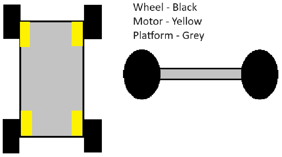
Mobile Platform on Wheels
A platform can move around by controlling its motors. The sensor will be mounted on the platform, enabling it to move across space.
The advantage of a wheeled platform is the ease of development and deployment. Building such a mobile platform and mounting a sensor on it is trivial, and many off-the-shelf solutions for a mobile platform may already exist.
However, there are limitations to this solution. The design of a wheeled platform is inherently flawed because its ability to traverse certain terrains is limited. The wheeled platform is only suitable for operating on roads and paths. Any other conditions, such as rugged landscapes, can limit platform mobility. This can lead to incomplete data collection as the platform might struggle to access critical pollution sources hidden in the terrain. Additionally, the platform's performance could be compromised in adverse weather conditions such as muddy or slippery ground. While solutions can overcome all these challenges, as seen with NASA's Mars rovers, they will be too impractical to implement, take too long to develop, and have overall complications.
Another disadvantage of the wheeled approach is the confinement of a specific space. A wheeled platform's movement is inherently limited by its distance and the speed at which it can reach various points within that space. Given the limitations in terrain, for a wheeled platform to move from point A to point B, it may need to take a detour even though point A to point B might be a straight line through some rough terrain. This means the spatial confinement limitations can affect the comprehensiveness and accuracy of air quality data collection, especially in scenarios where pollutants disperse over large areas.
Pollutants will spread depending on wind patterns, topography and location of the pollution source. A wheeled platform's limited mobility might hinder its ability to capture these dispersion patterns over significant distances. Moreover, the limited speed of the platform can impact the efficiency of data collection, leading to delayed or incomplete readings. Multiple wheeled platforms must be deployed across space to mitigate these limitations. However, this introduces additional complexity regarding coordination, synchronisation, and data integration from the sources.
A key requirement of the sensor is for it to be mobile on the z-axis. This means a mechanism must lift the sensor up and down. However, there are challenges in lift height and practical constraints. The lift's height becomes a limiting factor in the maximum altitude at which data can be collected. Suppose the lift height is insufficient to reach the desired monitoring altitude. In that case, the platform's effectiveness in assessing pollution at certain heights is compromised. Furthermore, even if the lift height is adequate, the dimensions of the lift become concerning. If we use a screw lift similar to those found in 3D printers, the height of the mobile platform will be the height the sensor can measure.
The mobile platform will approximate a human's height if we want to measure air quality at human head height. This will make the platform design bulky and unwieldy. Further scaling this approach to reach higher altitudes becomes increasingly challenging. Another lift design is the scissor lift. However, this design will also introduce new complexities. Extending the lift's reach will either require longer scissor arms or more scissors. This will contribute to added weight and compromise the platform's manoeuvrability.
In conclusion, the limitations of a wheeled platform are the inability to traverse across different terrain, the distance it can travel and the cumbersome nature of lifting the sensor on the z-axis. Fortunately, all these issues could be addressed with a drone.
Drone/Quadcopter
A quadcopter is a highly manoeuvrable aerial vehicle with four rotors. The quadcopter, such as the air quality sensor, can carry a substantial payload.
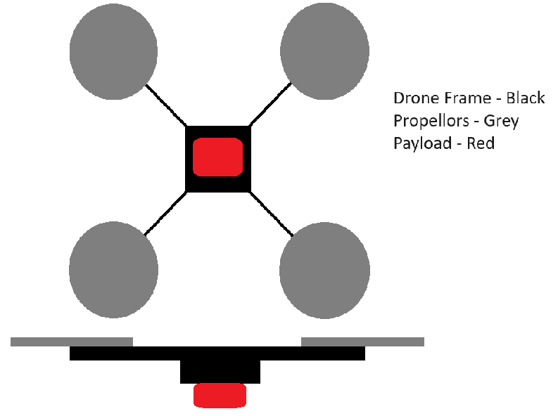
The advantage of a quadcopter is that it mitigates most of the problems experienced by a wheeled platform. The quadcopter can effortlessly navigate in the z dimensions. It does not require intricate lift mechanisms and can rapidly ascend and descend, allowing it to capture data at various altitudes. Furthermore, a quadcopter can reach altitudes as high as it wants, given that it is within regulation and hardware limits. This means it could provide insights into pollution that ground-based sensors cannot capture.
A quadcopter also is fast. They can cover large distances in shorter time frames, making them well-suited for monitoring air quality across expansive areas. Furthermore, quadcopters are not limited by the terrain as they fly over them. This versatility starkly contrasts wheeled platforms, which might struggle with specific geographies, limiting their access to critical pollution sources. A quadcopter can provide a more accurate representation of air quality across ample space.
A drawback of using a quadcopter is the air disturbance caused by the drone's propellers. The air currents generated by the propellers could alter the surrounding air composition, potentially affecting the accuracy of air quality measurements. However, this concern needs to be evaluated in context. By comparing the resultant air quality data with data gathered beforehand, it is possible to assess the significance of this disturbance. If there are significant disturbances, then a solution to mitigate such disturbances is required. Otherwise, a relationship may be extrapolated, and the "incorrect" air quality readings could be converted into an approximate value.
Another potential limitation arises from a drone's payload capacity. Depending on the size and hardware of the quadcopter, there might be constraints on the weight of the sensors and equipment it can carry. This could limit the number of sensors deployed on the drone, affecting the air quality measurements. To address this issue, one can use more powerful motors or consider using lighter and more compact sensor technologies to reduce the payload weight.
Development
Why DIY Drone?
From the previous analysis, a drone is more suitable for making the air quality sensor mobile. While buying an off-the-shelf drone and securing the air quality sensor within budget constraints is possible, the drone will not have significant payload-carrying capacity. Furthermore, there will be no software integration between the drone and the sensor unit.
A DIY drone kit will be used. These kits typically include all the essential components necessary to construct a functional drone, simplifying the process and eliminating the need to source parts individually and check for compatibility. Furthermore, there are many guides online, reducing the development time.
Most DIY drones use the open-source Ardupilot platform. The MAVLink protocol allows external devices to communicate with the flight controller. This means the Arduino in the air quality sensor can pull GPS data from the GPS module of the drone, and the drone can respond appropriately depending on air quality measurements.
Refer to Appendix D for more details on the building of the quadcopter.
Integration
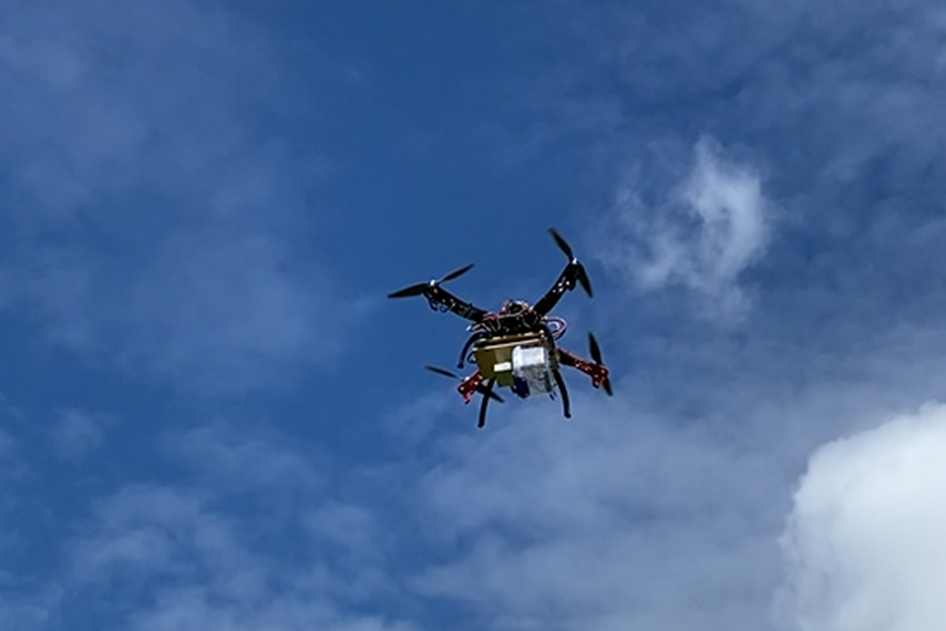
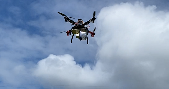
The images below highlight the final solution, with the air quality sensor integrated into the drone.
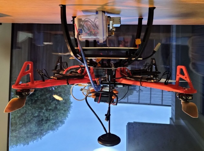
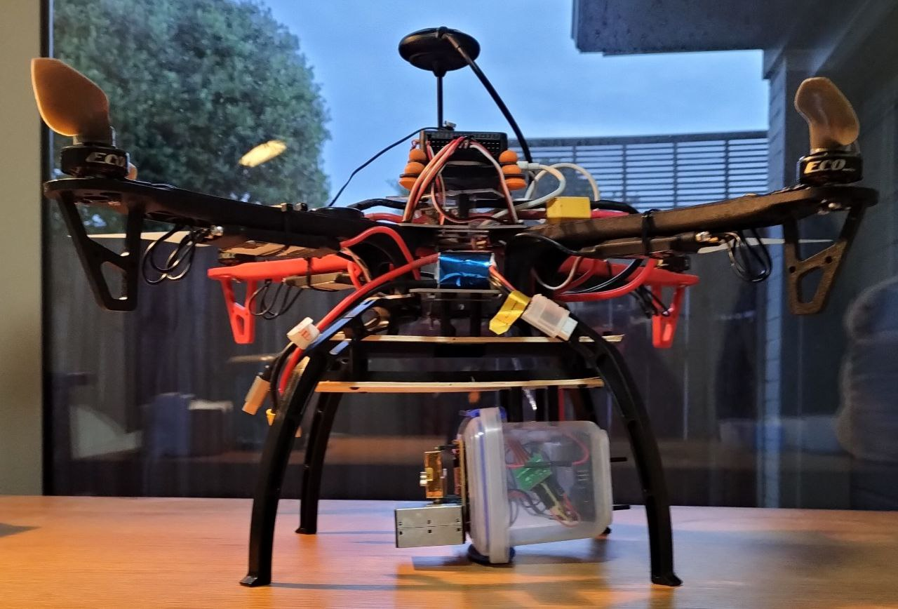
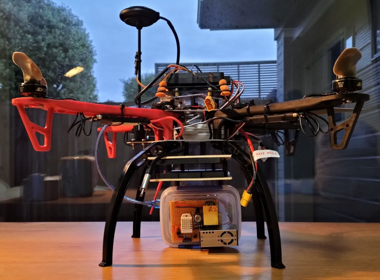
The link and the QR code will point to a brief video of an explanation of the mobile air quality sensor and a demonstration of it in flight: https://youtu.be/x9GDhE7BiPA

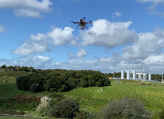
Testing
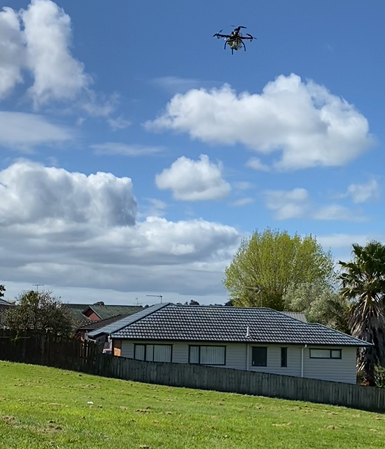
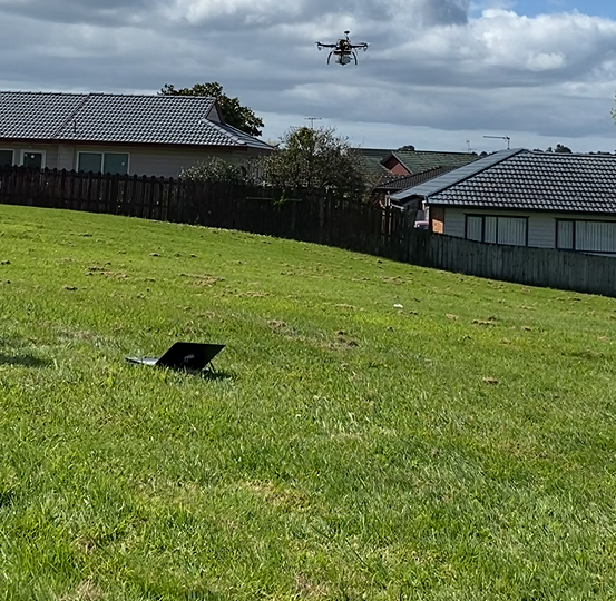
The images below show the mobile air quality sensor flying.
Deployment
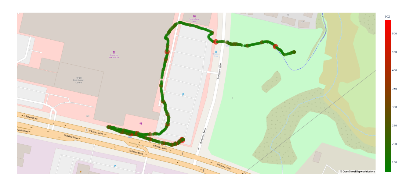
The drone captured the air quality of outdoor spaces: near congestion, next to the hardware store and the nature reserve. As seen in the graphs, there are variances in air quality. Unlike the section "Are There Air Quality Variances in Space?", the only difference is that all readings are done remotely from the drone. The following paragraphs will analyse the specific characteristics of the data gathered.
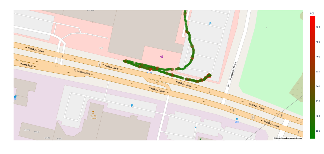
As the image above shows, the road next to Ti Rakau Drive has periodic bad air quality readings. This is because the high concentrations of cars due to congestion will emit more pollutants, resulting in higher PCI values. Upon reviewing video footage of the drone flying, the periodic extreme readings are attributed to when the drone passes by trucks and buses, diesel engine vehicles. The literature confirms these readings: "diesel vehicles cause more than four times the pollution than petrol cars" (Nieuwenhuis and McNabola). The PCI increases approximately four times when diesel engine vehicles pass. The data gathered by the drone shows high spatial resolution data that a single sensor could not achieve, in this case, extreme changes in air quality at localised spaces.
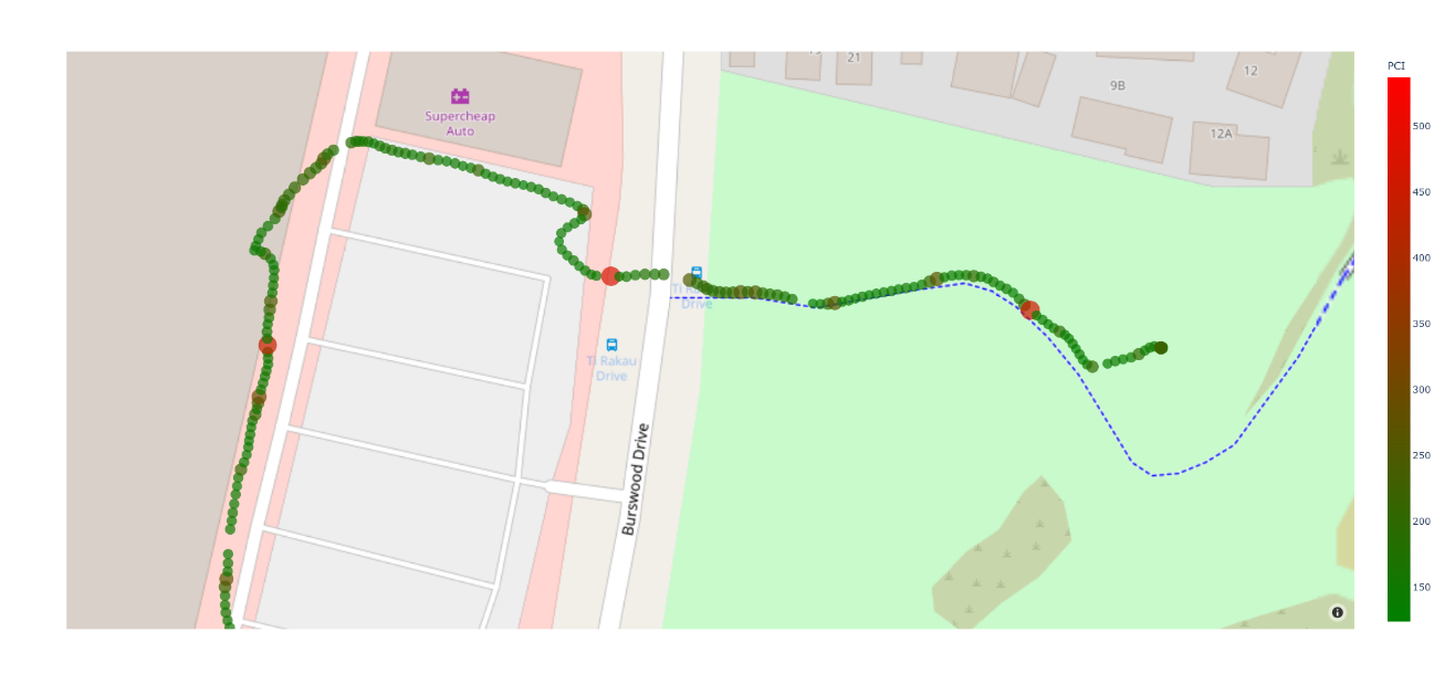
The hardware store from the image above is the same as in the section "Are There Air Quality Variances in Space?" The air quality remains relatively constant, apart from the occasional increase in PCI. This is attributed to the fact that it is the parking space -- the increase in PCI results from cars parking or leaving the parking spaces. Furthermore, there is one point with a significant increase in PCI. The hardware store's space for woodworking is open; therefore, the particulate matter will diffuse out, which is picked up by the sensor. Supporting this idea is the fact that the air quality outside the auto parts store is relatively good. Since the auto parts store has no ventilation, it contributes to the abnormal readings inside the building. However, it also means all the VOCs cannot diffuse into the surroundings, so the outside air is good.
Finally, there are two points with high PCI. As the drone flew across the street and to the nature reserve, it passed by some flowering trees. The pollen from the trees meant the drone detected high particulate matter concentrations, resulting in a high PCI.
Evaluation
Feedback
I contacted Najam Haq, who runs the Young Engineers Workshop. He specialises in these types of electronic projects. Thus, his knowledge and feedback helped me develop the project faster and better. The following is the feedback he gave me.
Feedback 1
Hi Ethan,
I had a look at the sensor module for your air quality logging drone. You still have quite a few sensing problems to solve, and it looks like you are running out of I/O lines on Arduino. You also have a power source problem; you'll have to supply the sensors and Arduino with a substantial power source. I have an idea that might solve multiple problems.
I recommend that you get rid of the SD card unit; that will free up some IO (the SD card has its own problems anyway; it is speed-limited on the Arduino, so it is easy to glitch it out and corrupt it). Instead, incorporate a modern phone into the unit. This will give you a power source -- phones have pretty substantial batteries in them and give you a place to log the data into; plus, you can also get some remote telemetry via the phone's data connection. For an Arduino serial connection to the phone, look up an app on Google Play called "blynk."
If you are on an iPhone, there is something equivalent available in the Apple store as well; you will have to search for it.
Let me know how it turns out. Good luck!
Najam
Feedback 2
Hi Ethan,
I had a quick read of your write-up, I have a couple of comments:
I think you are piling too many technical nitty-gritty details into your main write-up, affecting the report's readability. I suggest you put low-level details in appendices and focus on your project's gist and high-level details in the main write-up. I think this will make your report more readable. Anyone who needs the details can always look things up in the appendix.
I think your PCI formula needs quite a bit of work. Combining multiple independent variables into a single variable is quite a tricky thing to do. I don't think your current formula is getting there.
Najam
Feedback 3
Hi Ethan,
Looks like things are coming along. Well done on the progress so far. It seems you are struggling with the enclosure for the unit. Sometimes, the smallest of things can be the biggest of pains. You could continue doing a 3D printed design, but I suggest you avoid this long turn-around design process. This is a prototype, a one-off design. I would focus on getting the unit airworthy rather than perfect in looks. The iteration time on 3D printing is too long; you should work directly on the platform with basic materials (plywood, acrylic, corflute sheets, glue, tape, velcro, zip ties). I am quite sure you'll get to the end quicker. Good luck!
Najam
Feedback 4
Hi Ethan,
Good job on how far you have come! I think this is going to be great; I am looking forward to seeing actual data coming out of this thing.
Regarding mounting sensors, I think one thing you should consider is interference from the drone's propellers and the drone's motion. You are measuring concentrations of particulate matter and gases. Rapidly moving air will tamper with all of these to some degree. I suggest you (a) mount the sensors facing down rather than horizontally (b) create a snorkel shroud for the sensor that collects air as far away from the drone as possible. You could probably just use the lightweight dryer vents you can get from Bunnings. This latter is usually telescopic. You can fold it when the craft is on the ground; it will naturally unfurl as the craft takes off.
Najam
Personal Reflection
I implemented most of Najam's feedback into the project and writeup. However, due to time constraints, his final feedback is left as future improvements.
More specifically, he advised limiting air interference due to the propellers by mounting the sensor pointing downwards and developing a shroud around it. However, a limitation of the drone frame is the relatively short legs, or conversely, the air quality sensor is still too large. There is not enough space to mount the sensors pointing downwards. It will take a non-trivial amount of time to order longer legs for the drone or design a robust one from scratch. Since the shroud idea depends on the sensor being mounted vertically (if we implement a shroud with the sensors pointing forward, there will be insufficient air intake), this idea is not feasible.
Furthermore, he questioned the soundness of the PCI formula. I agree that the current formula of doing a weighted sum to calculate the PCI mathematically does not make sense. Upon further reading, a better model will use a piecewise linear function. For readings of the same units, for example, different particulate matter size concentrations, a weighted sum can be used to quantify the particulate matter air quality. However, the PCI should follow a proportionality when combining this with temperature, humidity, CO2 and VOC readings with certain limits. A better model might be \(\text{PCI} = k \times \text{CO2} \times \text{VOC} \times \text{PM} \times \text{temperature} \times \text{humidity}\), where \(k\) is a proportionality constant, and the values of the sensor readings are input into some function where values below and above a certain threshold will cap out at a maximum and minimum value. For example, it does not matter if CO2 levels are at 5000 PPM or 7000 PPM as both these values are deadly, so any value above 5000 PPM will be given a score of 10. However, determining the function for the acceptable ranges of values and how different measures are combined is complicated and requires further research. Thus, developing a more sound PCI model is a key undertaking.
Improvements
However, I believe these improvements are beyond this project's scope. The goal of the investigation was to prove there are air quality variances and develop a solution to overcome the limitations. Despite the simplistic PCI formula, it does show the variance of air quality in space, although the value is potentially meaningless. Analysing the raw data shows that each sensor recorded significant fluctuations in readings across space. Thus, the conclusion remains unaltered. There are substantial variances in air quality within space. The improvement will be to quantify these fluctuations into a single value. Finally, the quadcopter and the corresponding data it gathered showed a potential solution for collecting high-resolution air quality data in an automated manner. In terms of the project, I believe it has fulfilled the primary goals of the investigation.
Appendix
A: Portable Sensor Unit
Component Research
Microcontroller
The role of a microcontroller in a sensor unit will be to read sensor data and save the data to an SD card. The Arduino family of microcontrollers, Raspberry Pi and NVidia Jetson are potential microcontrollers worth considering.
The microcontroller has several requirements:
- Low power consumption. Due to space limitations in the final miniature solution, the chosen microcontroller will prioritise low power consumption. While an external supply can power a prototype, any feasible final design will not have sufficient room to accommodate an ample supply. Therefore, designing a system that requires low power consumption during the prototyping phase is crucial.
- Small form factor.
While Arduinos, Raspberry Pis, and NVidia Jetsons offer compact options, Raspberry Pis and NVidia Jetson devices resemble lightweight personal computers, featuring WiFi connectivity, multiple USB ports, and HDMI ports. They require an operating system to be installed on their storage drive, and these additional features contribute to increased power consumption. In contrast, Arduinos are suitable options as they only execute the program stored in their EPROM. They are low-level boards with minimal built-in IO, allowing for the addition of relevant sensors and IO specific to the sensor unit. This approach reduces both the monetary cost and power consumption.
Temperature and Humidity Sensor
There are two temperature and humidity sensor variants, DHT11 and DHT22. Both these sensors contain a capacitive humidity sensor and a thermistor.
A capacitive humidity sensor operates on changes in the capacitance of a material when exposed to moisture. When humidity increases, moisture is absorbed by the dielectric material, causing it to increase in volume. There is a change in distance between the two conductive plates. Capacitance is inversely proportional to the distance of the conductive plates, so depending on humidity levels, capacitance varies. By measuring the capacitance, humidity can be determined after calibration.
A thermistor operates based on changes in its electrical resistance with temperature. It consists of semiconductor material. When temperature changes, the movements of charged particles within the semiconductor lead to changes in its conductivity, which affects the flow of current, leading to a change in resistance. The resistance of a thermistor is inversely proportional to temperature. By measuring the resistance, the temperature can be determined after calibration.
The table below highlights the key differences between these two models.
| DHT11 | DHT22 | |
|---|---|---|
| Humidity Accuracy | 20%-80% humidity readings, ±5% accuracy | 0%-100% humidity readings, ±2.5% accuracy |
| Temperature Accuracy | 0-50 degrees, ±2 degrees accuracy | -40-80 degrees, ±0.5 degrees accuracy |
| Sampling Rate | 1 Hz | 2 Hz |
While the range of humidity and temperature readings is sufficient for the DHT11, the accuracy of DHT22 is significantly higher. Since the sensor unit is required to detect minor variances in space nearby, it demands high precision from the sensors. The sampling rate is not a problem as one reading per second differs from two readings per second as the humidity and temperature do not fluctuate drastically within this period.
From this brief analysis, it could be concluded that the DHT22 is the superior temperature and humidity sensor.
CO2 Sensor
There are two main CO2 sensors, MG811 and the MHZ-XX model. Both these sensors operate differently.
The MG811 adopts a solid electrolytic cell principle. A redox reaction occurs in the electrochemical cell when exposed to CO2. This generates an electromotive force by Nernst's equation \(E = E^{\circ} - \frac{RT}{zF} \ln(Q_c)\). The greater the CO2 concentration, the greater the electromotive force produced. By measuring the electromotive force, CO2 concentration can be determined after calibration.
The MHZ-XX family of sensors uses infrared absorption to detect CO2. An infrared source illuminates gas inside the measurement chamber. Some wavelengths get absorbed by the gas. An optical detector detects the unabsorbed wavelengths. Since the infrared spectrum of CO2 is unique, it is possible to identify the presence of this gas by matching the detected wavelengths with the expected wavelengths, otherwise known as fingerprinting. The CO2 concentration levels can be calculated by the intensity of the light reaching the detector. The intensity of light is inversely proportional to CO2 concentration.
The table below highlights the key difference between these two sensor models.
| MG811 | MHZ-XX | |
|---|---|---|
| Range | 350-10000 ppm | 0-10000 ppm (model dependent) |
| Accuracy | No data | ±50 ppm |
| Response Time | No data | <90, <120 (model dependent) |
| Preheat Time | No data | 1-3 minutes (model dependent) |
| Ideal Operating Conditions | 25°C ± 2°C, 65% ± 5% humidity | No data |
Range-wise, there are no significant differences between these sensor moduli. However, since the MG811 measures CO2 concentration by the chemical properties of CO2, the effectiveness of such reactions will have a range. There is a range of ideal operation conditions. Since this proof of concept is trying to measure variances in air quality, some spaces will inevitably fall out of the ideal operating conditions of the MG811, making this sensor unsuitable. On the other hand, since MHZ-XX sensors measure CO2 concentrations based on the physical properties of CO2, the physical properties of CO2 will remain constant for the temperatures that will be measured.
As noted above, there are various models of the MHZ-XX family of sensors. The table below highlights the key differences between them.
| MH-Z14 | MH-Z14A | MH-Z14B | MH-Z19B | MH-Z19C | |
|---|---|---|---|---|---|
| Ranges | 0-5000 ppm | 0-10000 ppm | 0-10000 ppm | 0-10000 ppm | 0-5000 ppm |
| Preheat Time | 3 minutes | 3 minutes | 30 seconds | 3 minutes | 1 minute |
| Response Time | <90s | <120s | <90s | <120s | <120s |
| Accuracy | ±50 ppm | ±50 ppm | ±50 ppm | No data | No data |
The MH-Z14B sensor is equal to or superior to other models in every category. From this brief analysis, it could be concluded that the MH-Z14B is the superior CO2 sensor.
VOC Sensor
Choosing an appropriate VOC sensor was challenging due to the vast number of models available and ways of implementation. There are three types of VOC sensors: electrochemical sensors, metal oxide sensors and photoionisation sensors. This paper will focus on the following models: MQ135, CCS811, BME680 and SGP40.
As the CO2 Sensor (MG811) mentions, an electrochemical sensor functions by a redox reaction, which occurs when electrodes are exposed to volatile organic compounds. The concentration of such compounds is determined by the voltage produced by the redox reaction.
A metal oxide sensor operates on the same principle as the thermistor. The resistivity of the metal oxide changes when the metal oxide is exposed to the volatile organic compound. The resistance of the metal oxide determines the concentration of the volatile organic compounds.
A photoionisation sensor uses the concept of the photoelectric effect. UV light emits high-energy photons, which the volatile organic compound absorbs. Consequently, the molecule gains energy, and an electron is ejected from the molecule, forming a positively charged ion. A small current, which can be amplified, is measured from the ejected electron. Volatile organic compound concentration can be determined by the current produced. However, it is essential to note that this sensor can also be affected by factors such as humidity, interfering gases, and lamp ageing, which may require periodic calibration and maintenance to ensure accurate measurements. Disregarding these factors, if ceteris paribus, the photoionisation sensor offers all sensor types the greatest response, accuracy and precision. However, a single sensor costs $800, which is out of budget. Thus, this type of sensor will not be considered in the following analysis.
The specifications of MQ135, CCS811, BME680 and SGP40 are different. Each sensor module contains differing additional features, such as temperature and humidity measurements for BME680 or integrated algorithms to consider environmental factors for SGP40 and CCS811. However, many of the additional features these sensors offer could be achieved through software and the integration of additional external sensors, which this air quality sensor unit will use. This means a fair comparison between sensor modules is impractical and unnecessary. The MQ135 is a basic VOC sensor without any additional functions, and its accuracy will be improved through the sensor integration with the DHT22. Consequently, the MQ135 is also the cheapest option.
Due to the presence of other sensors, it is possible to use an inferior sensor as the other sensors in the air quality sensor unit will compensate for it. Therefore, the MQ135 will be used due to lower costs.
Particulate Matter Sensor
The particulate matter sensor measures particulate matter. There are two different versions of particulate matter sensors: the PMS family of sensors and the DSM501 dust sensor. Both of these sensors operate in the same way.
As air actively passes through the sensor, it will pass through a laser light, typically in the infrared or visible spectrum. The particulate matter will interact with the light in such a way that results in the scattering of the light, otherwise known as Mie scattering. The intensity of Mie scattering is dependent on the particle size. A larger particle will result in more significant scattering. A photoelectric sensor detects such scattering and returns the concentration of the sampled air.
A comparison table is not required for this analysis as the DSM501 has a significant shortcoming of no factory calibration. This means any air quality reading from this sensor will only qualitatively indicate whether a space has good air relative to prior measurements. This project should avoid manual calibration, considering its focus on high-precision measurements. Attempting to calibrate the sensor independently may introduce unforeseen errors, particularly in the context of the non-optimal air quality within the calibration spaces. Furthermore, the DSM501 does not have a fan to actively pull air, which means the volume of air it samples will be inconsistent.
As for choosing which PMS family of sensors, the datasheet specifies that the accuracy and precision of the PMS5003 and PMS7003 are the same; however, the PMS7003 was redesigned to be thinner and draw less power. Consequently, the newer generation means a higher monetary cost; thus, the PMS5003 will be used for this project, albeit with a greater power draw and slightly larger dimensions.
Real-Time Clock
A real-time clock is a clock that is independently powered by the microcontroller, so it continues to track the time even if the microcontroller is off. There are no specific requirements for a real-time clock, so whichever model was available was used.
SD Card Reader
An SD card reader can read and write on an SD card. In this case, the SD card reader will write the data from the microcontroller to an SD card so that the data can be logged and processed later. There are no specific requirements for an SD card reader, so whichever model was available was used.
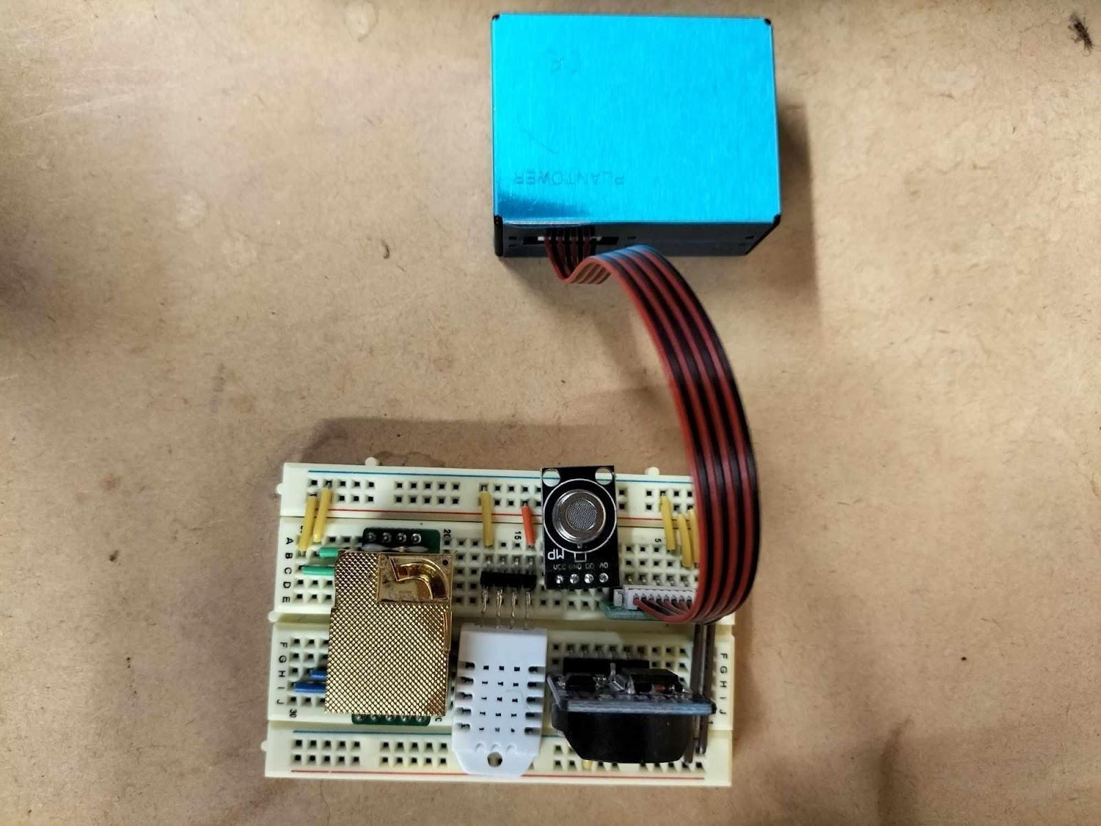
Individual Sensor Testing
Before making a more robust design, testing each sensor is essential. This can be easily achieved by mounting the sensors on a breadboard. As for the code, pre-written libraries would speed up development time.
The following paragraphs document the issues encountered during this phase of development.
Issue: Particulate Matter and CO2 Sensor Not Working Individually
A recurring issue with the particulate matter sensor during testing was that the sensor failed to provide any readings, only to mysteriously start working after a few weeks and then stop working again.
Various troubleshooting steps were taken to address this problem. By trying a different sensor, it is possible to determine whether or not it was a sensor fault. However, the replacement sensor also exhibited the exact behaviour. Thus, the problem was something else. Another possibility was a software bug, so different libraries were tried, yet the behaviour continued.
Upon further investigation, the root cause of both sensor malfunctions was an elementary misunderstanding regarding the serial communication protocol. Serial communication involves transmitting data between devices via the sending device's transmitter (TX) pin and the receiving device's receiver (RX) pin.
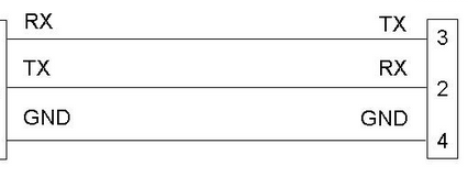
The problem was the incorrect assumption that, like regular input/output ports, the RX and TX pins should be wired to identical pins between devices. The CO2 and particulate matter sensor had the RX pin connected to the RX port and the TX pin connected to the TX port on the microcontroller. Serial communication requires a cross-wiring approach, with the transmit pin of one device wired to the receive pin of the other and vice versa. During component testing, the wiring was sporadically wired "incorrectly" and ironically led to the right results. This explained the periodic results.
Issue: Particulate Matter and CO2 Sensor Not Working Together
While the example code for each sensor worked flawlessly, they did not work together. This was a limitation in the SoftwareSerial library. The SoftwareSerial library allows communication on other digital pins of an Arduino board through emulation, allowing the Arduino to interact with multiple sensors using the serial protocol. However, the library allows for only one instance of serial communication. It was not possible to use two sensors using serial protocol through the SoftwareSerial library.
However, the Arduino has a dedicated serial port (hardware serial). By assigning one of the two sensors to the hardware serial port, only one sensor will use the SoftwareSerial library. However, a drawback of utilising the hardware serial port is that it shares the same bus with the USB connection. Conflicts arose during the upload of code. The hardware serial pin had to be disconnected during upload and later reconnected. While this solution works, it is inconvenient due to the additional steps involved.
Issue: Serial Buffer Overflow
To illustrate this problem, a simpler pseudo-code will be used. When printing the data individually, for example:
print(PARTICULATE_MATTER_DATA)
print(CO2_CONC_DATA)
print(TEMPERATURE_DATA)
it would output:
1, 2, 3
300
25
This is expected behaviour. However, for better data parsing later, the data was formatted like this as a string variable first before printing the variable:
string = String("PM: " + PARTICULATE_MATTER_DATA + "CO2: " + CO2_CONC_DATA)
print(string)
Unfortunately, this did not output the desired format of PM: 1, 2, 3 CO2: 300 but rather PM: 1, 2, 3 C???????.
The problem was the Arduino's memory limitation and the String class' implementation. The String class creates a copy of the original string literal and allocates dynamic memory for it at runtime. Therefore, both the original string literal and the dynamically allocated string coexist in memory. If the original string stores many bytes, the Arduino may run out of SRAM. As a result, data in the string variable becomes corrupted.
Furthermore, the serial buffer overflowed due to the immediate display of the many bytes of data, resulting in data loss and unsuccessful printing. To resolve this, unnecessary text was removed, reducing the size of the data sent through the serial port. Furthermore, smaller chunks of the string were printed, resulting in the desired format while working within the memory constraints.
Prototype
Robust Installation
After confirming that each sensor works together, a more robust attachment method is required, as the breadboard is only for prototyping. The sensors were soldered to a Veroboard, reducing the risk of loose connections or intermittent failures.
Issue: Wire Connections
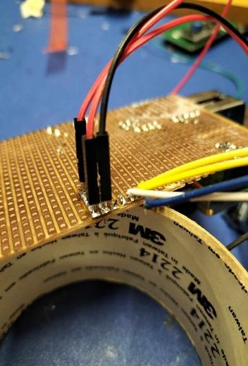
An issue arose when attempting to create connections between the Veroboard and the Arduino. Initially, a male Dupont wire was cut. One end was soldered to the Veroboard, and the other side was plugged into the Arduino. However, the thin exposed wires were prone to breakage. The male header was directly soldered onto the Veroboard instead of cutting the male Dupont wire to address this. This approach eliminated the vulnerability of the fragile wires.
The image illustrates the problem and the solution. On the right side of the image, the blue wire is detached from its solder joint, while the white wire is breaking. On the left side of the image, the revised approach shows no signs of breakage.
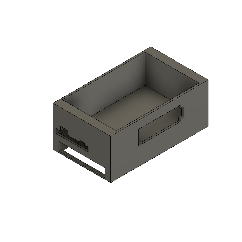
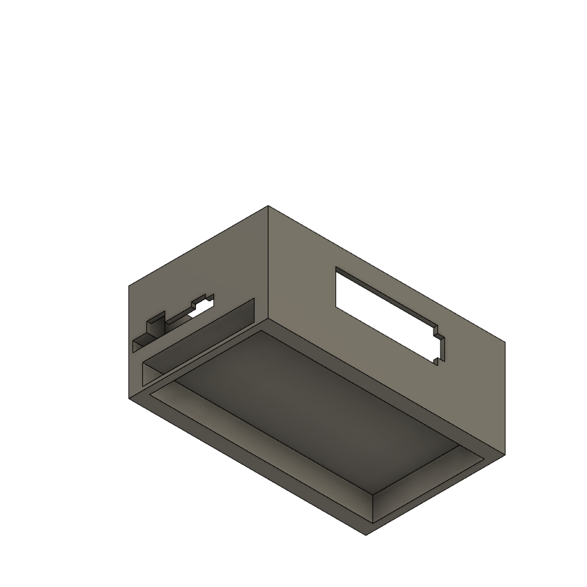
Enclosure Design
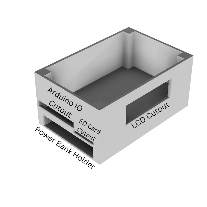
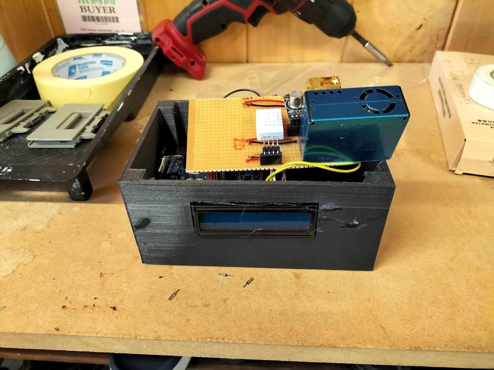
The enclosure was designed using Fusion360 and 3D printed. It was intended to contain the sensors and a power bank. The diagram illustrates the enclosure's design and each cutout's functions.
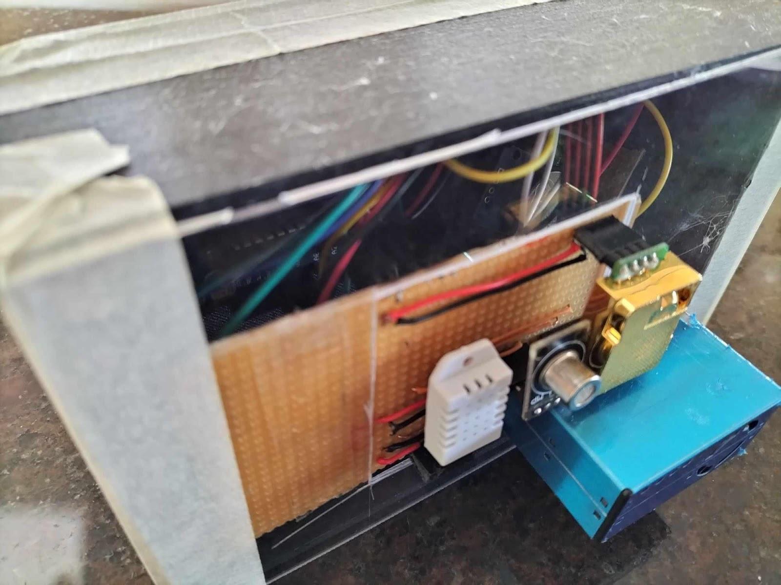
The photos below highlight how each component fits inside the enclosure.

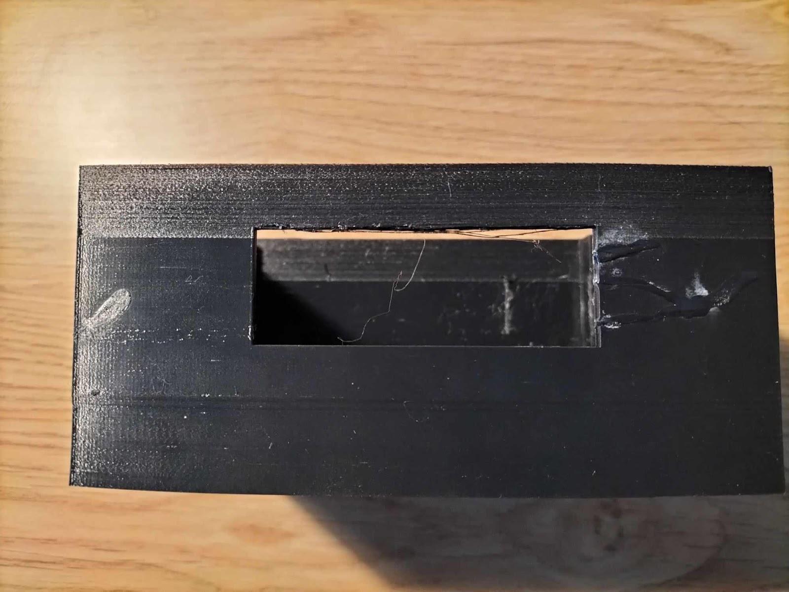
Issue: Incorrect Dimensions
Due to measurement errors, the dimensions of the Arduino IO cutout were incorrect. Therefore, plastic was cut out from the enclosure to create sufficient space, as seen in the picture below.
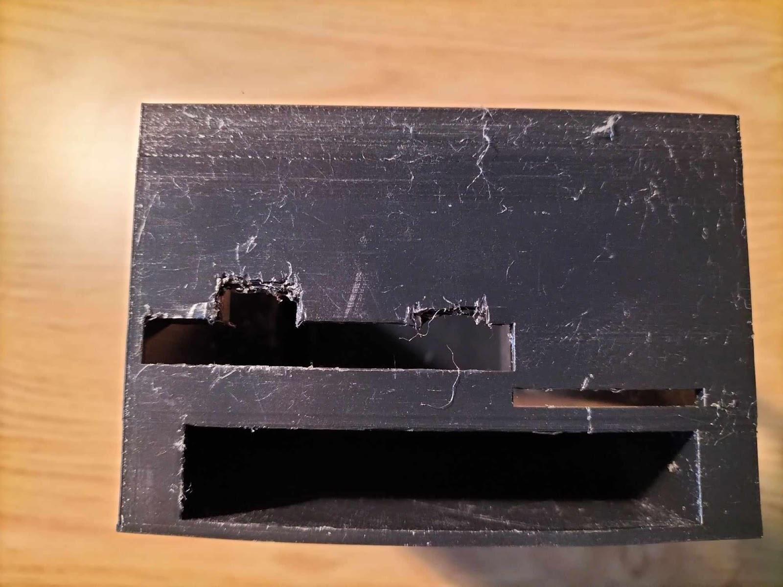
Furthermore, the design did not account for a notch on the LCD module. This prevents the LCD from being mounted flush.
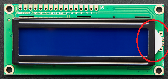
However, cutting out plastic for the LCD notch cracked the case. Therefore, the cracks were superglued, and it was decided to temporarily deal with a misaligned LCD until the next enclosure design iteration.
Modifications were made to account for the measurement errors and allow the components to fit together correctly within the enclosure. This enclosure's future designs will be modified in CAD accordingly before printing.
SD Card Reader Integration
Issue: SPI, Serial and I2C Protocol Conflict
The SD card reader caused issues. Appending a "write to SD card" function to the code prevented everything else from working. The conflict was attributed to the use of the SoftwareSerial library.
To address this issue, the SoftwareSerial library was switched to AltSoftSerial. This library was chosen based on its compatibility with the SPI (SD Card) and Serial (Sensors) protocols. However, this resulted in the real-time clock and the LCD module to stop working. Both these components use the I2C protocol. The documentation mentioned, "some libraries may disable interrupts for longer than 1-bit time. If they do, AltSoftSerial will not work properly." It was hypothesised that the issue lay in the warning from the documentation.
Without any clear solution, a complete pivot was made in the project. Instead of using an SD card reader, the sensor unit was redesigned to connect the Arduino to a mobile phone via an OTG (On-The-Go) connector. This resulted in an unexpected externality. There was no need for an SD card reader, and the phone has timestamp logging capabilities and provided power to the Arduino via USB. This meant the power bank and the real-time clock were no longer required.
Furthermore, since the phone supports multitasking, the phone can log data with respect to time. At the same time, another application would use the GPS sensor in the phone to log the phone's location with respect to time. Now, the air quality measurements could be matched to geolocation by comparing the times.
Final Prototype
To address the previous design flaws and the change in the architecture of the sensor unit, a redesign was undertaken.
The image below shows the following modifications to account for the previous incorrect measurements. Additional cutouts accommodate the Arduino IO and a tab for the LCD module. Furthermore, the cutout for the SD card was removed.
The image below shows a cutout in the battery holder part to allow for visibility of the phone screen during operation.
The Veroboard was attached to a piece of polycarbonate sheet, which was taped on the top, and the phone cutout also had a polycarbonate layer to prevent the phone from falling out of the box.
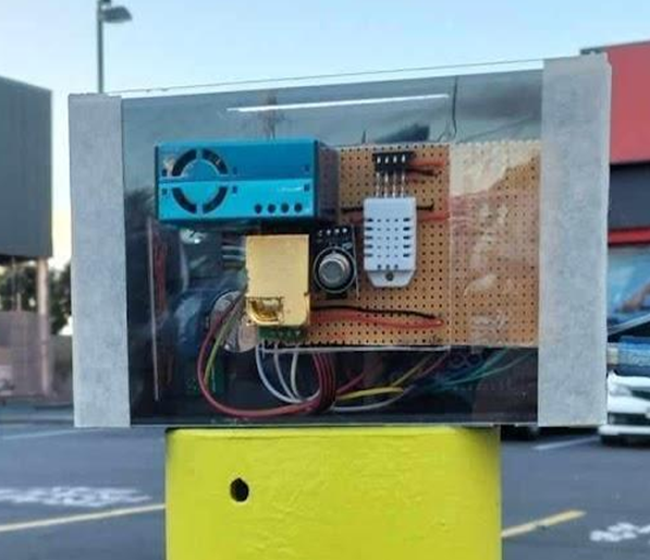
The images below show the final prototype of the sensor unit.
B: Data Gathering and Processing
Since the data gathering and processing stages were happening in parallel, the method of data gathered at home and processed will be different than at the hardware store, which will also be different than at school. The data processing pipeline gradually refined as data was gathered from different locations. This will be discussed during the data processing section.
Data Gathering
As mentioned in the "Are There Air Quality Variances in Space?" data will be gathered by continuously running the sensor while moving around. The Serial USB Terminal app records the data. One interesting feature of this app is the dedicated logging feature, which adds timestamps to each data log. This means the real-time clock is redundant, simplifying the sensor unit.
Matching the location and the data log for the first two investigations, at home and a hardware store, a map of the locations was subdivided into sections.
The image below shows that the hardware store is divided into sections.
The image below shows how the sensor moved through the hardware store. Each large section is subdivided into smaller subsections and numbered. Since we know where the sensor is at all times, the timestamps can be manually noted at each section. For example, in section one, the data recorded will be between the time stamps of 10:00 and 10:01.
While this method worked for the home measurements, this method does not scale up. Notifying down the time stamps and planning a predetermined path for every space takes too much time. The time taken to record the measurements of the hardware store was one hour.
However, the phone which is logging data also has a GPS. By recording timestamped GPS coordinates from the phone, it is possible to match the sensor data with location information. The Phyphox app logs GPS coordinates against time, and the data can be exported. The phone supports multitasking, so Phyphox and Serial USB Terminal will run simultaneously. This method saved much time, as recording the measurements at school only took twenty minutes.
Data Processing
How the data was processed for analysis depended on how the data was gathered.
At home, there was a small number of data points. Therefore, an Excel spreadsheet was used to calculate the pollution concentration index.
However, this method will not work for the data gathered at the hardware store. The data collected is continuous; therefore, the data needed to be somehow separated according to the corresponding timestamps by each section. A Python script was created to do this separation automatically. The user will input their desired timestamp range, and the script will modify the data accordingly. In this case, the script will highlight the sections in red.
from openpyxl import load_workbook
from openpyxl.styles import PatternFill
from datetime import datetime

def get_times(file):
    times = []
    with open(file) as f:
        startchunk = False
        f = list(f)
        for i, line in enumerate(f):
            lin = line.split()
            if not startchunk:
                time1 = lin[0]
                startchunk = True
            if lin == []:
                time2 = f[i-1].split()[0]
                times.append([time1, time2])
                startchunk = False
    return times

def modify_excel_file(location_file):
    times = get_times(location_file)
    wb = load_workbook(filename="output.xlsx")
    ws = wb.active
    redFill = PatternFill(start_color='FFFF0000', end_color='FFFF0000', fill_type='solid')
    for cell in ws['A']:
        for time in times:
            time1 = datetime.strptime(time[0], '%H:%M:%S.%f')
            time2 = datetime.strptime(time[1], '%H:%M:%S.%f')
            if(type(cell.value) != str):
                if time1.time() <= cell.value <= time2.time():
                    cell.fill = redFill
    wb.save("processed.xlsx")

def func(location_file, data_file):
    times = get_times(location_file)
    with open(data_file) as f:
        f = list(f)
        for i, line in enumerate(f):
            for time in times:
                time1 = datetime.strptime(time[0], '%H:%M:%S.%f')
                time2 = datetime.strptime(time[1], '%H:%M:%S.%f')
                check = datetime.strptime(line.split()[0], '%H:%M:%S.%f')
                if time1.time() <= check.time() <= time2.time():
                    print(line, "A POINT")
                else:
                    print(line, "NOT A POINT")

if __name__ == "__main__":
    func("outdoors.txt", "raw.txt")
    modify_excel_file("outdoors.txt")
However, this method still requires manual work. Since each section is highlighted, it serves as a marker for a human to manually create graphs on each section. As mentioned earlier, this still takes time and will not scale up as the space size increases.
All of this was greatly simplified after using timestamped GPS coordinates. A Python script could read the GPS and recorded data timestamps, combine them, and save them in a separate file. Utilising GPS coordinates obviates the necessity of partitioning the measured space into distinct sections, as each recorded GPS point inherently represents its self-contained section. Furthermore, Python libraries allow the coordinates to be plotted on a map. The possibilities are limitless. For this case, each point will be given a colour and size. The colour represents the relative pollution concentration index. The more red the colour, the greater the pollution concentration index, while the more green the colour, the better the air is.
The following code combines the timestamps into one file.
import pandas as pd
from datetime import datetime, timedelta
import re
import utm

location_file = "school.xls"
air_data_file = "school.txt"

location = pd.ExcelFile(location_file)
location_data = pd.read_excel(location, "Raw Data")

location_data["PCI"] = -1
location_data["Temperature_(C)"] = -1
location_data["Humidity_(%)"] = -1
location_data["VOC_(PPM)"] = -1
location_data["CO2_(PPM)"] = -1
location_data["PM1.0_(ug/m3)"] = -1
location_data["PM2.5_(ug/m3)"] = -1
location_data["PM10_(ug/m3)"] = -1

time_data = pd.read_excel(location, "Metadata Time")
start_time = datetime.strptime(
    time_data["system time text"][0].split(" ")[1], "%H:%M:%S.%f"
)

with open(air_data_file, "r") as file:
    text_lines = file.readlines()

for i, timestamp in enumerate(location_data["Time (s)"]):
    location_time = (start_time + timedelta(seconds=timestamp)).replace(microsecond=0)
    location_data["Time (s)"][i] = location_time

    for data in text_lines:
        data_time = datetime.strptime(
            data.split(" ")[0], "%H:%M:%S.%f"
        ).replace(microsecond=0)

        if location_time.time() == data_time.time():
            parsed_data = data.split()
            location_data["Temperature_(C)"][i] = float(
                re.sub("[^0-9.]", "", parsed_data[2])
            )
            location_data["Humidity_(%)"][i] = float(
                re.sub("[^0-9.]", "", parsed_data[4])
            )
            location_data["VOC_(PPM)"][i] = float(
                re.sub("[^0-9.]", "", parsed_data[6])
            )
            location_data["CO2_(PPM)"][i] = float(
                re.sub("[^0-9.]", "", parsed_data[8])
            )
            location_data["PM1.0_(ug/m3)"][i] = float(
                re.sub("[^0-9.]", "", parsed_data[10])
            )
            location_data["PM2.5_(ug/m3)"][i] = float(
                re.sub("[^0-9.]", "", parsed_data[12])
            )
            location_data["PM10_(ug/m3)"][i] = float(
                re.sub("[^0-9.]", "", parsed_data[14])
            )
            location_data["PCI"][i] = (
                0.05 * location_data["Temperature_(C)"][i]
                + 0.2 * location_data["Humidity_(%)"][i]
                + 0.5 * location_data["VOC_(PPM)"][i]
                + 0.1 * location_data["CO2_(PPM)"][i]
                + 0.7 * location_data["PM1.0_(ug/m3)"][i]
                + 0.4 * location_data["PM2.5_(ug/m3)"][i]
                + 0.3 * location_data["PM10_(ug/m3)"][i]
            )

location_data = location_data[location_data["PCI"] != -1]
location_data.to_excel(
    location_file.split(".")[0] + "_modified.xlsx", index=False
)
The following code plots the combined data on a map.
import plotly.express as px
import pandas as pd

location_file = "house_modified.xlsx"
location = pd.ExcelFile(location_file)
location_data = pd.read_excel(location, "Sheet1")

color_scale = [(0, 'green'), (1, 'red')]

fig = px.scatter_mapbox(
    location_data,
    lat="Latitude (°)",
    lon="Longitude (°)",
    hover_name="PCI",
    hover_data=[
        "Temperature_(C)", "Humidity_(%)", "VOC_(PPM)",
        "CO2_(PPM)", "PM1.0_(ug/m3)", "PM2.5_(ug/m3)", "PM10_(ug/m3)"
    ],
    color="PCI",
    color_continuous_scale=color_scale,
    size="PCI",
    zoom=8,
)
fig.update_layout(mapbox_style="open-street-map")
fig.show()
The code produces graphs that look like this:
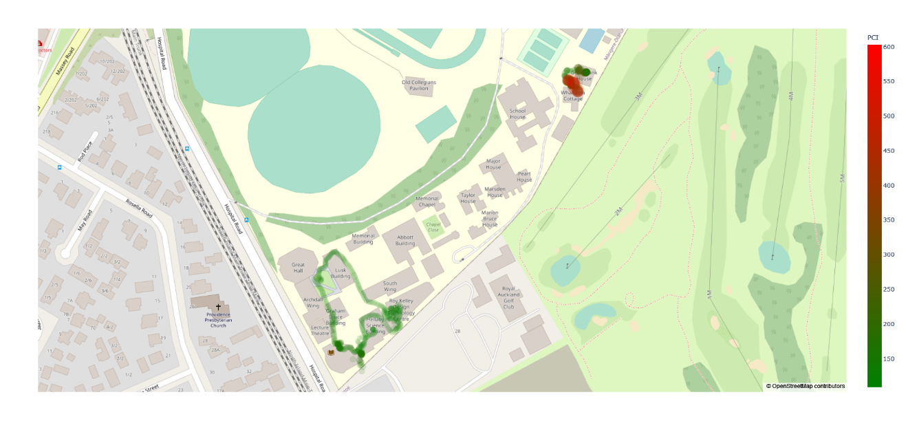
This data pipeline requires no human input. It is fully automated. All subsequent data recorded by walking around with the sensor or using the mobile air quality sensor will use this data pipeline.
C: Iterative Design Process
High-Resolution Measurements
Description
If the significant limiting factor of spatial resolution was the number of sensors, an obvious solution would be to increase the number of sensors in space. Scaling this idea to maximise spatial resolution and maintain temporal resolution would lead to filling an entire room with a sensor to measure every cubic unit of space every second.
Advantages
The most significant advantage of this solution is that it effectively overcomes the limitations of the current practices. The spatial resolution is maximised.
Cost Analysis
Eight thousand eight hundred eighty-eight sensors are required to measure every cubic unit of space in an average indoor room (calculated by average room volume / effective sensor coverage). Assuming that the wire length required to connect each sensor to a microcontroller mounted on a wall will be the length of the sensor to the wall, the total length of the linkage is 378m. Therefore, the total calculated monetary cost is $960,398.35.
The deployment time of this sensor mesh would be prolonged as a technician would have to fit 8888 sensors into a room and space it correctly. Furthermore, this solution interferes with useable space as all the sensors will take up the room entirely, shutting down the room during measurement and for a while longer for people to uninstall the sensor mesh so that the room can become usable. However, ironically, aesthetics is not a problem as no one would use the room to care about its appearance.
In terms of technical costs, if one wants to use WiFi to transmit data, it will not be possible. Assuming that the sensor mesh can use all the 2.4 GHz, 5 GHz, and 6 GHz bands, 376 bands will be available, significantly less than the 8888 required per sensor. Furthermore, storage cost is no longer negligible to maintain the same temporal resolution as the current practice. If a sensor records temperature, humidity, CO2, particulate matter and volatile organic compound data, and each data is a 32-bit integer, each sensor records 160 bits per second. The sensor mesh records 160 x 8888 bits/second or 177.76 KB/second. Therefore, one day of recordings will produce 122.87 GB of data, and one year will produce 44.85 TB.
Furthermore, this solution also has negative externalities. For example, the fact that there are so many sensors in a room might interfere with airflow, and the heating effect from all the sensors may result in inaccurate readings. Since inhabitants are not in the room, this solution will not accurately represent the air with people inside.
Reflection
This solution exemplifies reductio ad absurdum, where the most logical solution results in exorbitant costs. Instead, this solution empathises that subsequent ideas will require balancing monetary cost, practicality and technical feasibility while achieving higher spatial resolution.
Sensor Grid Drops Down
Description
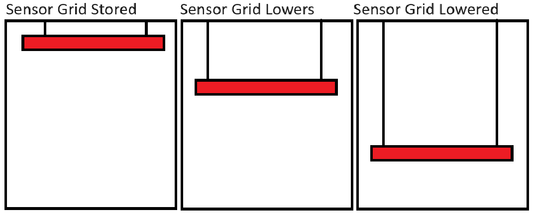
The most effective way to reduce the costs associated with the high-resolution measurement solution is to reduce the number of sensors deployed. However, this means each sensor must cover a greater volume to achieve the spatial resolution as the high-sensor-count solution. Since each sensor unit coverage volume is fixed, the only way for it to cover greater volume without sacrificing spatial resolution is for it to be mobile. An approach to this objective involves employing mobile sensors within a grid arrangement. This grid will be suspended on the room's ceiling and can descend and ascend using a winching mechanism. This allows for fewer sensors to cover the same volume of space.
Advantages
There are a few noteworthy advantages of adopting this mobile sensor grid system. Firstly, it achieves comparable spatial resolution to the prior solution, which occupies less physical space. Moreover, the winching motion of the sensor grid means the sensor would gather continuous spatial data rather than discrete point data; thus, it can be argued that spatial resolution along the z-axis may improve. However, the greatest advantage lies in the substantial reduction of sensors required by orders of magnitude, leading to a drastic reduction in monetary cost.
Cost Analysis
Based on the specified assumptions, the sensor mesh requires 888 sensors, calculated by dividing the ceiling area by the adequate sensor coverage. Each sensor module requires a minimum of three meters of linkage, corresponding to the average room height. As a result, the estimated monetary cost of this solution amounts to $97,534.79. The cost of this solution has been reduced by a factor of 10 compared to the prior solution. However, deploying this sensor grid is expected to be time-consuming as a technician needs to install a ceiling-sized grid on the roof. Additionally, during operation, the winching motion of the system will impede usable space; the consequences of such were discussed earlier. The greatest contrast between this and the prior solution is that during the operation of this sensor grid, it will be hanging on the ceiling, as opposed to the prior idea where it had to be completely disassembled. While there will be a reduction in technical cost as only a single installation is required without disassembling, from an aesthetic standpoint, a mounted sensor grid on the ceiling during operation may not be visually appealing. Regarding technical costs, using WiFi to transmit data will still be impossible as the 888 sensors are greater than the 376 WiFi channel bands available. It is also important to note that this solution is unsuitable for outdoor measurements.
Reflection
The observed monetary, practical and technical costs can still be attributed to this idea's high number of sensors. However, as discussed in the "Proof of Concept" section, while there are air quality variances indoors, they are minor. Therefore, data can be extrapolated. This means the sensor count can decrease even more.
Sensor Grid in Walls
Description
A more efficient approach to extrapolate the data will be strategically placing nine sensors per wall and reducing the frequency at which the data is gathered. Implementing a sensor grid on the four walls allows for a more streamlined and cost-effective data collection process.
Advantages
The primary advantage of this approach is the fewer sensors, making it more cost-effective. Furthermore, it does not interfere with the usable space in the room, and the installation process is relatively easy. Since the sensors are fixed, they provide a reasonable indoor spatial resolution for most applications. Additionally, by reducing the number of sensors, the data gathered per unit time decreases; thus, it is possible to increase the temporal resolution, given the same data storage space.
Cost Analysis
The proposed solution offers a cost-effective approach with a total cost of $3889 (36 x $108.35). The cost of the necessary linkages is negligible and not included in the calculation. However, installing sensors on the walls of a room, even with a reduced number, may still be considered impractical and aesthetically unappealing. This solution completely solves the technical issues. The reduced sensors mean there are enough WiFi channels to transmit data, and data storage is nearly negligible. However, this solution still does not work for outdoor measurements.
Reflection
To address the spatial resolution limitations posed by fixed sensors without increasing sensor count, a potential solution could involve delocalising the sensors and making them mobile. Like "Sensor Grid Drops Down", the movement of the sensors within space will provide high-resolution data. However, the delocalised nature of the sensor means the quantity of the sensor can decrease and use extrapolation to predict the air quality.
Crowdsourcing
Description
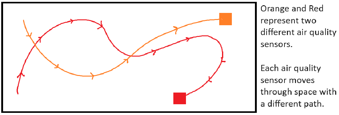
By attaching air quality sensors to individuals, as the individuals move, air quality data will be gathered in different locations, creating an air quality map.
Advantages
This strategy eliminates the need to measure air quality in vacant areas, optimising data collection. Furthermore, this solution allows for scalability. More participants mean finer data resolution. The non-intrusive nature and minimal spatial impact make it a practical choice.
Cost Analysis
Monetary costs are directly proportional to the number of participants (n). The overall cost is $108.03 x n. Linkage costs are minimal. Swift deployment arises from the seamless assimilation of sensors into daily routines. The allocated bandwidth proves adequate, contingent upon the number of sensor-endowed individuals.
However, a potential challenge lies in user fatigue from prolonged sensor carriage. Furthermore, the approach demonstrates diminished spatial and temporal resolution due to the inherently erratic trajectories of individuals. Moreover, the participants are susceptible to suboptimal air conditions during data collection. Furthermore, this method exhibits constraints regarding vertical coverage.
Reflection
Crowdsourcing solves many of the issues previously mentioned in other solutions. However, there will be inconsistencies due to the human nature of this solution. The way people move will determine what data will be gathered. Furthermore, since data is only gathered where people are going, it means the people wearing the air quality device will inadvertently be exposed to harmful air for public data.
The simplest way to overcome these problems will be automating the data collection. Suppose a robot could instead move around and take measurements. In that case, the locations where air quality is sampled will be consistent, and humans will not be involved in the process, saving time and money.
Automated Mobile Air Quality Sensor
Description
The solution employs a robot to gather data in different locations, creating a spatial air quality map. Otherwise, it is the same as crowdsourcing.
Advantages
This solution has all the advantages of crowdsourcing. However, in an automated way, it is not dependent on the human factor. This eliminates all the disadvantages exclusive to crowdsourcing.
Cost Analysis
The expense associated with implementing an automated mobile air quality sensor surpasses that of crowdsourcing but remains markedly lower than alternative solutions. However, it can be contended that over time, costs diminish owing to the inherent economising effects of robotic systems. Since this is a high-level overview of a concept, the actual cost of the solution may vary depending on how it is implemented.
Reflection
This solution will likely not be deployed indoors as it will interfere with usable space. However, this issue is negligible since this project only considers outdoor spaces.
D: Drone
Parts Selection
A DIY drone requires these parts to function minimally, excluding the frame: flight controller, electronic speed controllers, motors, propellors, GPS sensor, and buzzer. The flight controller contains other sensors, such as accelerometers and gyroscopes.
As for the reason why the specific parts were chosen, the main limiting factor was the cost and what was already available. The development of the drone was allocated $300; thus, components were chosen that would maximise feature count per unit cost. Furthermore, some parts, such as the motors, battery, propellors, remote controller and receiver, were already available. Therefore, parts that needed to be brought had to accommodate and be compatible with the existing components. All parts are sourced from Aliexpress to save cost.
Flight Controller
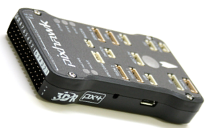
There are two main types of flight controllers: APM2.8 and Pixhawk 2.4.8. The main difference is that the Pixhawk has newer, more powerful and efficient components at the expense of the cost.
Initially, the APM2.8 would be the flight controller of the drone. However, upon reading the documentation, the latest software no longer supported this model. A workaround would be using an older software version, which means any fixed software bugs will not be reflected. Consequently, the Pixhawk 2.4.8 was chosen as the flight controller. However, the additional cost meant that the quality of the drone frame had to be compromised.
Building The Drone
The following paragraphs document the issues encountered during this phase of development. For the most part, building the drone was following the instruction manual.
Issue: Telemetry
Drone telemetry is the data gathered about the aircraft and is sent back to the operator. Telemetry is a prerequisite, and the drone cannot fly without telemetry. The drone kit did not come with a dedicated telemetry radio. Therefore, a workaround must be used. There is a service called Andruav. It uses the phone to act as telemetry. While regular telemetry will transmit radio signals, which will be received by a receiver attached to a laptop, Andruav instead connects the flight controller to the phone. Since the phone has a mobile network connection, it uses the internet to send telemetry data to the laptop. This resulted in an unexpected twist where long-range telemetry is possible. Regular radio-based telemetry only has an effective distance of one kilometre. Now, hypothetically, it is possible to control the drone anywhere.
The issue is that if the phone is connected to the flight controller, it is impossible to connect it to the mobile air quality sensor. As explored earlier, the Arduino from the air quality sensor can integrate directly with the flight controller, and it is possible to use the MAVlink protocol to send the air quality data along with telemetry data to the laptop. However, further research yields that this is an undocumented process. While hypothetically possible, no one has attempted it. Even for those who have attempted to do this, the conclusion of every post was essential to "write your software drivers for each individual sensor to make it compatible with the MAVlink protocol" (Rage et al.; Sheikh et al.) Attempting this is too complex, especially when the results are unproven.
Fortunately, using a USB hub solves this problem. This solution means the phone can receive data from the flight controller and the air quality sensor. While we cannot use GPS data from the drone, one must remember that we still have GPS data from the phone. By running three simultaneous applications, Andruav for telemetry, Phyphox for GPS logging and USB Serial Terminal for data logging, all the data is available and can be processed by the same data pipeline mentioned in Appendix B.
Issue: Incompatibility Between Frame and Antivibration Platform
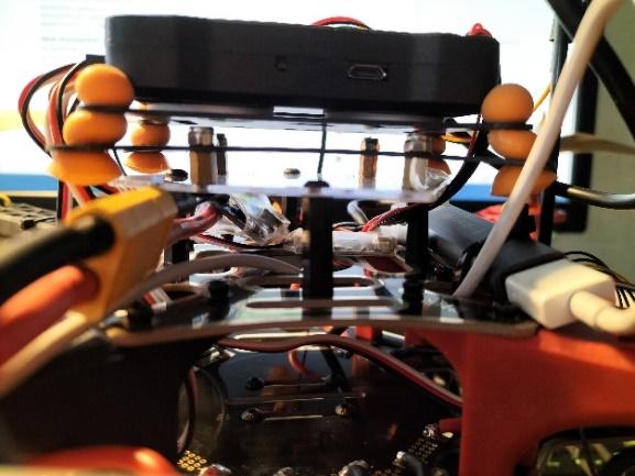
An antivibration platform mounted on the frame will prevent the flight controller from vibrating as much due to the motors. This means that the sensor data will not be as noisy. However, there was a misalignment of mounting holes with the frame. While a 3D-printed adapter seemed logical, the 3D printer was not operational. Instead, cutting a piece of polycarbonate and drilling the adapter holes yielded the same result. Standoffs also provided the necessary spacing for screws, eliminating direct contact between the screws and the flight controller. Ironically, this problem led to an unexpected benefit. The solution required to solve the problem also increased the free space in the drone, allowing for more efficient cable management.
Issue: Antivibration Platform Deterioration
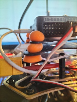
The antivibration platform contains four blue silicon feet. However, they were found to be susceptible to tearing. This created a weak point in the build, and if the feet entirely tore off, the flight controller would detach from the drone frame. A simple solution was to replace the feet with earplugs. The compressible and expandable attributes of the earplugs meant they were resilient against tearing, ensuring the durability of the assembly while upholding the requisite vibration-damping functionality.
Issue: GPS Sensor Wiring
The GPS sensor was discovered to be configured for an older model of the flight controller. This meant the pin arrangement was incompatible. Therefore, the pins had to be repositioned and swapped to align with the newer flight controller configuration.
Issue: Barometer Not Discovered in Software
The Pixhawk schematics are readily accessible and open-source, allowing manufacturers to produce diverse iterations of Pixhawk flight controllers. Consequently, it becomes plausible for specific Pixhawk models to incorporate sensor configurations that deviate from the specifications of the official variant. In the specific context of Pixhawk 2.4.8, its integration entails the utilisation of the MS5611 barometric sensor. An unforeseen complication surfaced wherein the prevailing flight controller firmware exhibited a bug, rendering it incapable of recognising this particular iteration of the barometric sensor. However, downgrading the firmware from 4.3.8 to 4.3.0 solved the issue.
E: MAQS (Integration)
To integrate the phone and air quality sensor into the drone, mounting holes are required to attach these components. Since modifications are required, this allows redesigning the following components. One critical design choice was to separate the phone holder component from the air quality sensor. This will create two independent modules, which allows greater flexibility on where to attach the components.
Phone Holder
Two pieces of plywood larger than the phone are cut out to create the phone holder. Then, holes were drilled to allow standoffs to be mounted so that the standoffs would act as a support to keep the phone in place to prevent it from moving sideways. The second piece of plywood also has the corresponding holes drilled out. The adhesive foam was also applied to the plywood to prevent the phone from getting damaged if an accident should occur.
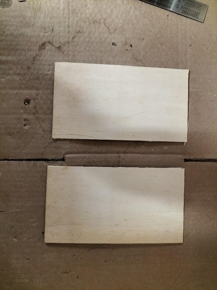
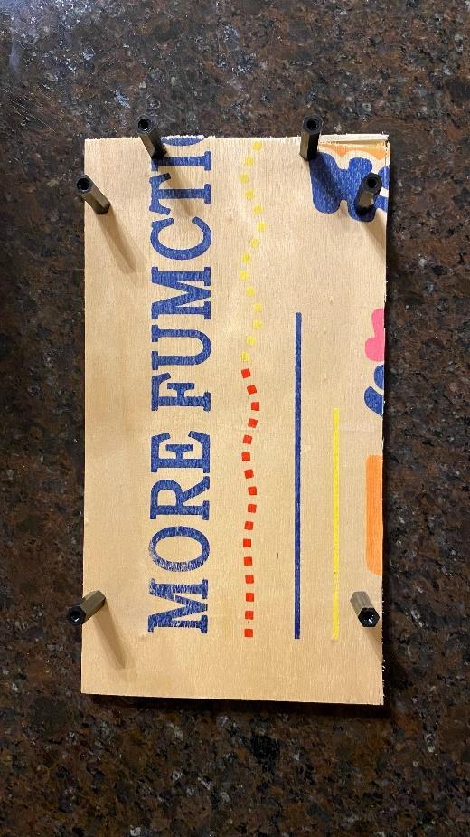
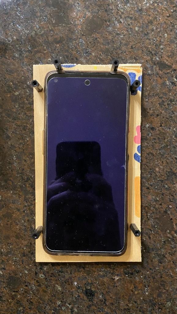
The image below shows the final phone holder design. The black standoffs circled in red are the standoffs attached to the drone.
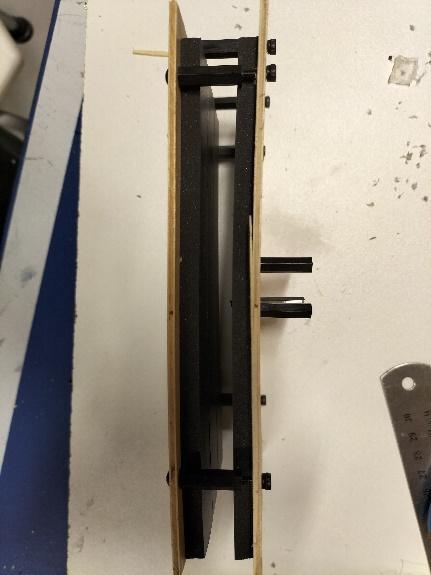
The screws used to secure the plywood to the standoffs are longer than necessary. This allows some leeway between the phone holder and the phone. The user can vary the clamping force on the phone, which allows easier accessibility in inserting and removing the phone from the holder. Furthermore, this design allows phones of various thicknesses to be used with the mobile air quality sensor.
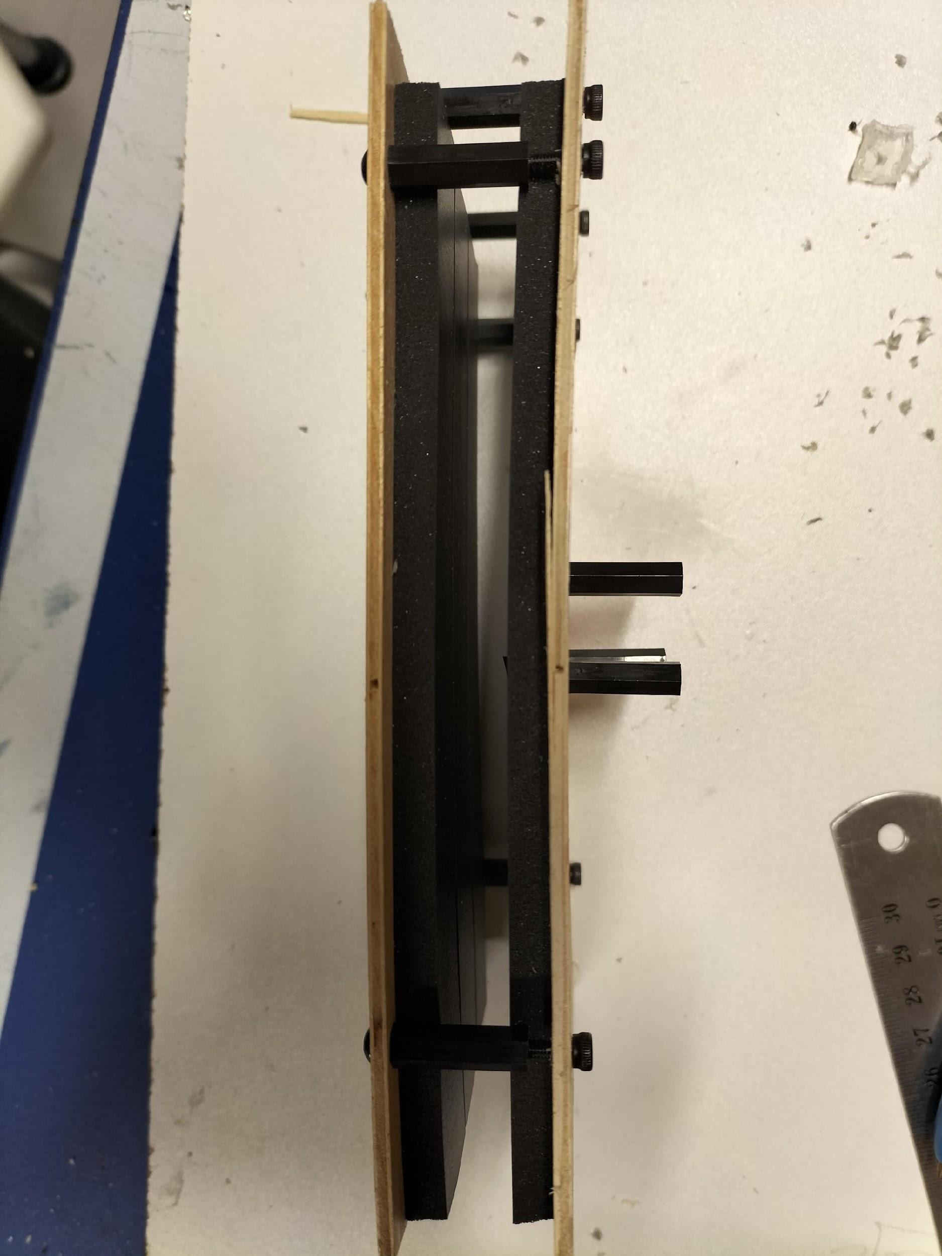
The images below show the phone holder attached to the drone.
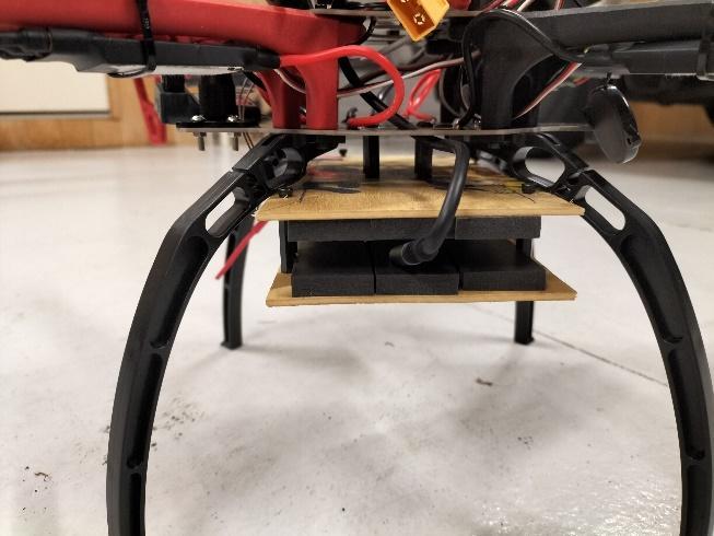
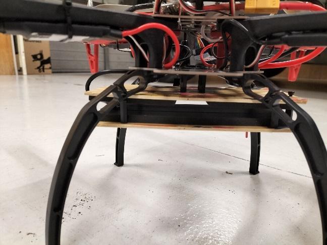
Air Quality Sensor
Appendix A shows the sensors attached to the box by masking tape. This is not a viable option, as the vibrations from the drone will cause the sensor to fall off. A robust solution is required. However, the 3D printer broke; thus, an alternative container design was required. A Sistema container was a suitable replacement. It was more compact than the prototype, but the clip-on lid meant that the internal components were still serviceable. All that was required was cutting through parts of the container to allow wires to pass through and using screws and nylon nuts to secure the sensors and Arduino to the container.
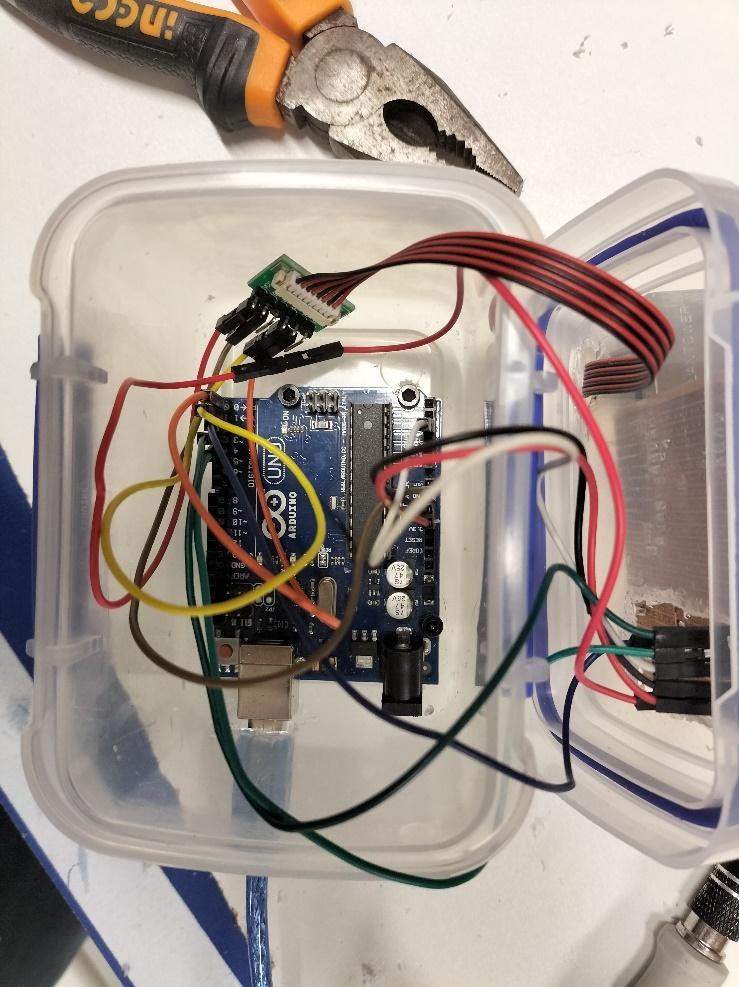
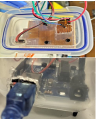
The Arduino fits inside the container. Holes were cut out to allow for wiring. The Veroboard was screwed down to the lid.
The image below shows the final version of the air quality sensor.
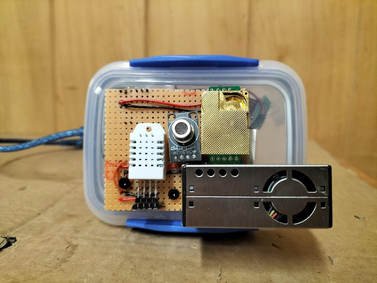
Like the phone holder, mounting holes were drilled out, and standoffs were used to mount the sensor onto the drone. The image below shows the mobile air quality sensor fully integrated.
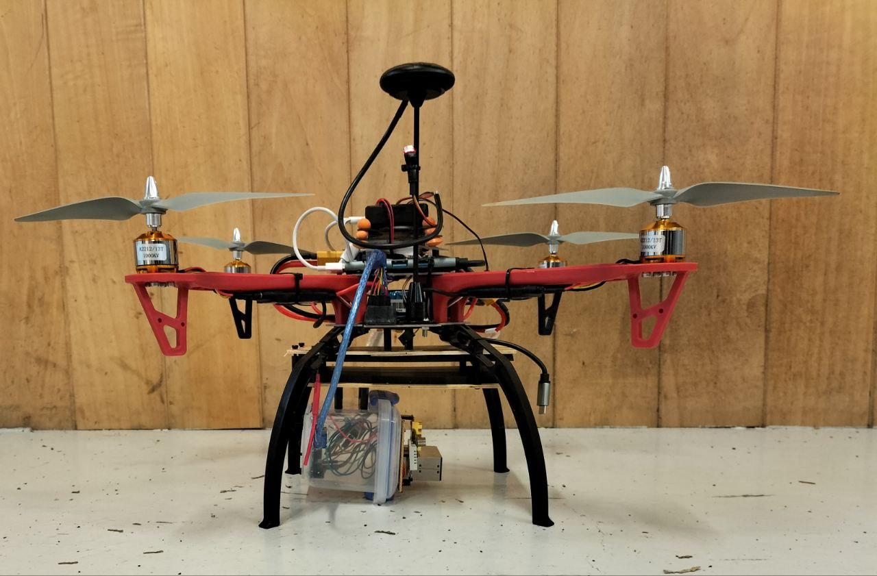
The air quality sensor was mounted to the drone's left. This was because, before the integration, the drone could not fly straight; it kept on tilting towards one side. It was suspected that the problem lay in the uneven weight distribution of the drone, with the GPS sensor to the front of the drone, causing it to tip forward. Therefore, the air quality sensor was mounted so that the heavier side would be on the opposite side, acting as a counterweight. Furthermore, the centre of mass of the air quality sensor was along the lid, so the mounting points were shifted to ensure that the centre of mass aligned with the drone, giving this off-centred mounted look.
Integration Problem
Despite the solutions mentioned above, the drone still could not take off. It turned out the motors used were too weak and faulty. On one motor, the shaft was not appropriately secured. Thus, the propellers could not spin to the designated rotations per minute. This was the cause of the tilting issue, as there is a resultant torque due to the difference in thrust provided by each motor. In hindsight, the motors should have been the first to check during diagnostics before concluding weight distribution. This is because Ardupilot, the software responsible for controlling the drone, comes with advanced control algorithms, like PID controllers, which allow the drone to stay upright. Once the shaft was secured, it was noted that the motors at full thrust could not lift the drone, so they were replaced with more powerful ones. The mobile air quality sensor worked after this fix.
References
- Aristodemou, Elsa, et al. "How tall buildings affect turbulent air flows and dispersion of pollution within a neighbourhood." Environmental Pollution, vol. 233, 2018, pp. 782-796.
- "Carbon Monoxide Poisoning." MyHealth.Alberta.ca Government of Alberta Personal Health Portal.
- "Children Are Dying from Air Pollution. Here's How We Can Protect Them." World Economic Forum.
- Education, UCAR Center for Science. "How Weather Affects Air Quality." Center for Science Education.
- "Electronic Smoking Devices and Secondhand Aerosol." American Nonsmokers' Rights Foundation, 18 Jan. 2023.
- "Health Effects of Air Pollution." EHINZ.
- "How Air Pollution Is Destroying Our Health." World Health Organization.
- "How Does Humidity Affect Air Quality? All You Need to Know." Airly.
- Lee, Suhyeon, et al. "Vertical measurements of roadside air pollutants using a drone." Atmospheric Pollution Research, vol. 13, no. 12, 2022, p. 101609.
- Manisalidis, Ioannis, et al. "Environmental and health impacts of Air Pollution: A Review." Frontiers in Public Health, vol. 8, 2020.
- Nieuwenhuis, Paul, and Aonghus McNabola. "Fact Check: Are Diesel Cars Really More Polluting than Petrol Cars?" The Conversation, 6 Oct. 2022.
- "Polluted Air Affects More than 90% of Children." UNFCCC, 29 Oct. 2018.
- Rage, Yuri, et al. "Unsupported Sensors? Try Arduino + Lua!" ArduPilot Discourse, 13 June 2022.
- Sheikh, Wamiq, et al. "I Want to Connect an Arduino with a Pixhawk via Serial Port." ArduPilot Discourse, 25 Apr. 2022.
- Terry Gibb, Michigan State University Extension. "Indoor Air Quality May Be Hazardous to Your Health." MSU Extension, 21 Jan. 2022.
- "Why Air Quality Matters." Ministry for the Environment, 3 Aug. 2021.
- Wiedinmyer, C., et al. "The fire inventory from NCAR (Finn): A high resolution global model to estimate the emissions from open burning." Geoscientific Model Development, vol. 4, no. 3, 2011, pp. 625-641.